Cross-posted from Riu’s blog.

In modelling disciplines, one often faces the challenge of balancing three often conflicting aspects: representational elegance, the breadth of examples to capture, and the depth or specificity in capturing those examples of interest. In the context of reinforcement learning theory, this raises the question: what is an adequate ontology for the techniques involved in agents learning from interaction with an environment?

Here we make a structural approach to the above dilemma, both in the sense of structural realism and stuff, structure, property. The characteristics of RL algorithms that we capture are their modularity and specification via typed interfaces.

To keep this exposition grounded in something practical, we will follow an example, Q-learning, which from this point of view captures the essence of reinforcement learning. It is an algorithm that finds an optimal policy in an MDP by keeping an estimate of the value of taking a certain action in a certain state, encoded as a table $Q:A\times S\to R$, and updating it from previous estimates (bootstrapping) and from samples obtained by interacting with an environment. This is the content of the following equation (we’ll give the precise type for it later):

\[\begin{equation} Q(s,a) \gets (1-\alpha) Q(s,a) + \alpha [r + \max_{a':A}Q(s',a') ] \end{equation}\]

One does also have a policy that is derived from the $Q$ table, usually an $\varepsilon$-greedy policy that selects with probability $1-\varepsilon$ for a state $s$ the action that maximizes the estimated value, $\max_{a:A}Q(s,a)$, and a uniformly sampled action with probability $\varepsilon$. This choice helps to overcome the exploration-exploitation balance.

Ablating either component produces other existing algorithms, which is reassuring:

• If we remove the bootstrapping component, one recovers a (model-free) one-step Monte Carlo algorithm.
• If we remove the samples, one recovers classical Dynamic Programming methods¹ such as Value Iteration. We’ll come back to these sample-free algorithms later.

The RL lens

Q-learning as we’ve just described, and other major RL algorithms, can be captured as lenses; the forward map is the policy deployment from the model’s parameters, and the backward map is the update function.

The interface types vary from algorithm to algorithm. In the case of Q-learning, the forward map $P$ is of type $R^{S\times A}\to (DA)^S$ (where $D$ is the distribution monad). It takes the current $Q$-table $Q:S\times A\to R$ and outputs a policy $S\to DA$. This is our $\varepsilon$-greedy policy defined earlier. The backward map $G$ has the following type (we define $\tilde{Q}$ in (2)):

\[\begin{align*} R^{S\times A}\times (S\times A\times R\times S) &\to T_{(s,a)}^{*}(S\times A) \newline Q, (s,a,r,s) &\mapsto \tilde{Q} \end{align*}\]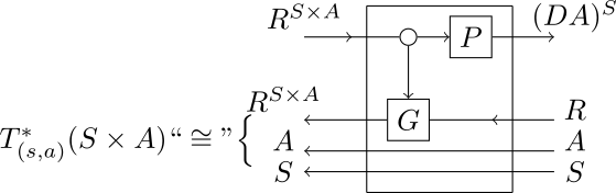

The type of model parameter change $\Delta(R^{S\times A})=T_{(s,a)}^{*}(S\times A)$ has as elements cotangent vectors to the base space $S\times A$ (not to $R^{S\times A}$). This technicality allows us to define the pointwise update of equation (1) as $((s,a),g)$, where $g=(r + \gamma\max_{a’:A}Q(s’,a’))\in R$ is the update target of our model. The new $Q$ function then is defined as:

\[\begin{equation} \tilde{Q}(\tilde{s},\tilde{a}) = \begin{cases} (1-\alpha)Q(s,a) + \alpha [r + \gamma \max_{a'} Q(s',a')] & (\tilde{s},\tilde{a})=(s,a) \newline Q(s,a) & o/w \end{cases} \end{equation}\]

The quotes in the diagram above reflects that showing explicitly the $S$ and $A$ wires below loses the dependency of the type $R^{S\times A}$ over them. This is why in the paper we prefer to write the backward map as a single box $G$ with inputs $R^{S\times A}\times (S\times A\times R)$ and output $T_{(s,a)}^{*}(S\times A)$.

From Q-learning to Deep Q-networks

Writing the change type as a cotangent space allows us to bridge the gap to Deep Learning methods. In our running example, we can do the standard transformation of the Bellman update to a Bellman error to decompose $G$ into two consecutive steps:

• Backward map:

  \[\begin{align*} G:R^{S\times A} \times (S\times A\times R\times S') &\to S\times A\times R \newline Q, (s,a,r,s') &\mapsto (s,a,\mathcal{L}) \end{align*}\]

  The loss $\mathcal{L}$ is defined as the MSE between the current $Q$-value and the update target $g$:

  \[\mathcal{L} = \left(Q(s,a) - g\right)^2 = \left(Q(s,a) - (r + \gamma \max_{a'} \bar{Q}(s',a')) \right)^2\]

  We treat $\bar{Q}(s’,a’)$ ($Q$ bar) as a constant value, so that the (semi-)gradient of $\mathcal{L}$ wrt. the $Q$-matrix is the Bellman Q-update, as we show next.

• Feedback unit (Bellman update):

  \[\begin{align*} (1+S\times A\times R)\times R^{S\times A} \to& R^{S\times A} \newline *, Q \mapsto& Q \newline (s,a,\mathcal{L}), Q \mapsto& \tilde{Q} \newline =& Q - {\alpha\over 2}{\partial\mathcal{L}\over\partial Q} \newline =& \forall (\tilde{s},\tilde{a}). \begin{cases} Q(s,a) - \alpha(Q(s,a) - g) & (\tilde{s},\tilde{a}) = (s,a) \newline Q(s,a) & o/w \end{cases} \newline & \forall (\tilde{s},\tilde{a}).\begin{cases} (1-\alpha) Q(s,a) + \alpha g & (\tilde{s},\tilde{a}) = (s,a) \newline Q(s,a) & o/w \end{cases} \end{align*}\]

  This recovers (2), so we can say that the backwards map is doing pointwise gradient descent, by only updating the $(s,a)$ indexed $Q$-value.

Continuations, function spaces, and lenses in lenses

Focusing now on sample-free algorithms, the model’s parameter update is an operator $(X\to R)\to (X\to R)$ between function spaces. State value methods for example update value functions $S\to R$, whereas state-action value methods update functions $S\times A\to R$ (the $Q$-functions). More concretely, the updates of function spaces that appear in RL are known as Bellman operators. It turns out that a certain subclass which we call linear Bellman operators can be obtained functorially from lenses as well!

The idea is to employ the continuation functor² which is the following representable functor:

\[\begin{align*} \mathbb{K} =\mathbf{Lens}(-,1) : \mathbf{Lens}^\mathrm{op} &\to \mathbf{Set} \newline {X\choose R} &\mapsto R^X \newline {X\choose R}\rightleftarrows {X'\choose R'} &\mapsto R'^{X'} \to R^X \end{align*}\]

The contravariance hints already at the corecursive nature of these operators: They take as input a value function of states in the future, and return a value function of states in the present. The subclass of Bellman operators that we obtain this way is linear in the sense that it uses the domain function in $R’^{X’}$ only once.

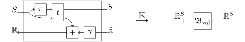
An example of this is the value improvement operator from dynamic programming. This operator improves the value function $V:S\to R$ to give a better approximation of the long-term value of a policy $\pi:S\to A$, and is given by

\[V(s) \gets \mathbb{E}_{\mkern-14mu\substack{a\sim \pi(s)\newline (s',r)\sim t(s,a)}}[r+\gamma V(s')] = \sum _{a\in A}\pi(a\mid s) \sum _{\substack{s'\in S\newline r\in R}}t(s',r\mid s, a) (r + \gamma V(s'))\]

This is the image under $\mathbb{K}$ of a lens ³ whose forward and backward maps are the transition function $\mathrm{pr}_1(t(-,\pi(-))):S \to S$ under a fixed policy $\pi:S\to A$, and the update target computation $(-)+\gamma\cdot(=):\mathbb{R}\times \mathbb{R}\to \mathbb{R}$ respectively, as shown below.

If you want to read more about this “optics perspective” on Value Iteration and its relation with problems like the control of an inverted pendulum, the savings problem in economics and more, check out our previous ACT2022 paper.

Once we have transformed the Bellman operator into a function using $\mathbb{K}$, this embeds into the backward map of the RL lens.

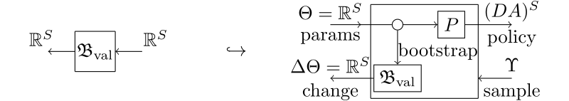
It is then natural to ask what a backward map that does not ignore the sample input might look like, and these are what we call parametrised Bellman operators. These are obtained by the lifting of $\mathbb{K}$ to the (externally parametrised) functor $\mathrm{Para}(\mathbb{K}):\mathrm{Para}(\mathrm{Lens}^\mathrm{op})\to\mathrm{Set}$, and captures exactly what algorithms like SARSA are doing in terms of usage of both bootstrapping and sampling.

Outlook

We talked about learning from bootstrapping and from sampling as two distinct processes that fit into the lens structure. While the difference between these two is usually not emphasized enough, we believe that it is useful for understanding the structure of novel algorithms by making the information flow explicit. You can find more details, along with a discussion on Bellman operators, the iteration functor used to model stateful environments, prediction and bandit problems as nice corner cases of our framework, and more on our recent submission to ACT2024.

Moreover, this opens up the study of stateful models: multi-step methods like $n$-temporal difference or Monte Carlo Tree Search (used e.g. in AlphaZero), which we will leave for a future post, so stay tuned!

---