From Equilibrium Checking to Learing with the Open Game Engine

Compositional game theory, like game theory in general, is not just for toy models. Game theory is the standard tool for modelling in a wide range of applications in microeconomics, and many of those benefit from compositionality. One of these applications is pricing, and especially its modern version, dynamic pricing. We have been working on a research project on how to do dynamic pricing in a strategic, competitor-aware way, using compositional game theory and its natural connections to optimal control and reinforcement learning, and building on the Open Game Engine.

In this post I’m going to discuss how we adapted the Open Game Engine, which is fundamentally designed as an equilibrium checker, to do multi-agent learning instead. The project we did also involved a lot of economics, which Nicolas wrote about in this post.

From equilibrium checking to dynamic programming

The idea that open games can be adapted to do dynamic programming has been known since 2019, when I replicated a dynamic social dilemma environmental economics model from Barfuss’ PhD thesis using the Open Game Engine (although that early implementation was very naive and almost melted my CPU before converging). A much more robust implementation, which used the Open Game Engine together with Python’s RLlib library, was built by Philipp and Nicolas (who I have been collaborating with on this project) for their paper on algorithmic collusion in pricing games.

At the time there was no theory explaining why this worked, that came slowly over the next few years. First there was Towards Foundations of Categorical Cybernetics (ie. the paper that really founded this field) revealing the full scope of open game-like constructions, and theoretically grounding all of the ways in which I was already creatively mis-using the Open Game Engine to do things it was not originally designed to do.

Then came the paper Value Iteration is Optic Composition, which fully explained the trick that I had used to do dynamic programming in the open game engine. In short, what that paper showed is that Bellman operators are representable as optics (both in the intuitive sense but also in the technical sense of representable functors), and that Bellman backup (ie. the application of a Bellman operator to a value function) can be justified as just precomposition with that optic. This operation, together with juggling the necessary indexing, is one of the main tasks that the computational backend of the Open Game Engine was built to do, since it is also what is needed for compositional Nash equilibrium checking.

The intuitive idea of how these things fit together can be explained with a diagram taken from Towards Foundations, the picture of a generic parametrised bidirectional process.

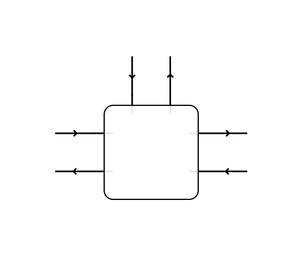
For a typical game-theoretic application the left and right boundaries have game states flowing forwards and payoff vectors flowing backwards, and they compose like bidirectional process, by backprop. The way we use this dimension for compositional modelling is unmodified from how we have always done it, so I will say nothing more about it here. For us, the interesting part is the top boundary.

The input on the top boundary is strategy profiles (which also goes by terms such as “parameters”, “policy” etc. depending on the application). The output on the top boundary, which I sometimes call “costrategies”, is the one that we need to focus on. On paper this output is a boolean value, and the different correctness lemmas for various classes of open games show that when the left and right boundaries are trivial, this value is true exactly when the input strategy profile belongs to some class of equilibria.

On one level, going from equilibrium checking to dynamic programming is as simple as changing this boolean to a real-valued payoff, and then attaching to the top boundary an optimiser that does policy improvement, ie. each loop iteration adjusting the policy in a way that increases that value. Since value improvement (ie. estimating the value of the current policy) is handled by the magic of optic composition in the horizontal direction, this is enough to give us dynamic programming.

We can also go beyond this, from dynamic programming to reinforcement learning. This is only a small step in theory but required a lot of details to be figured in practice, which appear in the paper Reinforcement Learning in Categorical Cybernetics.

Now let’s look at how all this looks in code.

A look inside the Open Game Engine

Let’s start with the most important definition in the Open Game Engine code base, the definition of open games themselves, and dissect it. The definition can be found here and looks like this:

data OpenGame o c a b x s y r = OpenGame
  { play :: a -> o x s y r,
    evaluate :: a -> c x s y r -> b
  }

(I have made one change from the linked code, which uses heterogenous lists instead of types a and b, an implementation detail that can be ignored in this post.)

There are several different minor variations of the definition of open games and the differences between them are understandably confusing. This version predates both this paper and this paper which significantly changed how we think about open games, but even so this version of the definition has stood the test of time extremely well.

The last 4 parameters - x, s, y, r - are the 4 legs of an open game. This post is not an introduction to how open games work, so if you want to understand this part you can go back to the original paper.

Next let’s talk about o and c, which from their use sites can be seen to take x, s, y, r as parameters. They range over typeclasses for optics and contexts respectively. The most basic example of such an o is o = Lens, which we use for game theory with deterministic (aka. pure) strategies, which could be imported from a library such as Control.Lens or simply defined concretely as Lens x s y r = x -> (y, r -> s). (The source code still uses the letters that I first wrote down in early 2015, years before I knew about lenses or the famous s t a b convention.)

The corresponding instance of contexts c that we use for basic game theory is c x s y r = (x, y -> r), which is also called Context in Control.Lens here. The structure that c has to satisfy is what I call a Tambara comodule, which I blogged about in this post.

For most serious game-theoretic modelling we use the definition of optics and contexts for Bayesian open games developed in this paper, which use existential types and can be found in the codebase here.

Now we come to the last two parameters, a and b, which are the important ones for this post. a is the type of strategy profiles of the open game. At this point we can read the second line of the definition, play :: a -> o x s y r, and say that an open game has an optic indexed by strategy profiles.

b is probably the point where what we do in the Open Game Engine differs most significantly from any version that has been written down on paper. On paper this is a boolean value that records whether the given strategy profile was a Nash equilibrium or not. What we use there in practice is a record type called DiagnosticInfo, which captures all available information about the decision, including the move that was played, that payoff received, the optimal move and payoff, the information that was visible and the information that was not visible. By looping the evaluate function over parameters and looking at the information contained in the returned record, a lot of microeconomic analysis is possible.

When modifying this output to be simply values, the basic decision operator that is the main generating element of real models - which is very complicated in a game-theoretic setting - becomes very simple and does nothing but shuffle values around, in particular forwarding the relevant payoff out of the top boundary to the optimiser. The code for that can be seen here. The reason for doing it this way is that the optimiser then lives outside of the open games framework, which means it can use unboxed arrays and other tricks in order to squeeze enough speed out of Haskell.

Learning in practice

For the past 6 months we have been working with a major airline on a pilot research project ¹ on strategic, competitor-aware dynamic pricing using this technology.

The game part of our model is a market, and the reason that compositional game theory is such a good fit is that the market for airline tickets has significant natural compositional structure due for example to connecting flights. This is precisely the point where we expect that our methodology will outperform traditional modelling. There is at least an entire blog post of things to say about this point alone, but that post will come later.

There are two very different ways we can proceed from there. The first way we can use it is to fix the strategy of one competitor (in our model a strategy is a policy for how a price varies dynamically over a time period) and then learn an optimal response for the other competitor. This puts us in a traditional dynamic programming setting, which is important because we get very strong convergence guarantees.

The other way to use it is to simultaneously learn both policies by multiagent RL, starting from some initial policies. This is another point where there is an entire blog post worth of things to say, but in short, there are few convergence guarantees but our experience is that the method usually works very well in practice. Fortunately, the complex issues we face here are not made any more difficult by using compositional game theory, so there is a lot of existing knowledge on multiagent learning that we can draw on.

All of this is to say that what I’ve been writing in this post is only one part of a much bigger research topic that includes significant amounts of computer science and economics (and I haven’t even mentioned the data science part). This very much fits into my overall vision for applied category theory as a field, where category theory makes its one contribution (ie. bringing compositionality to a new domain) and then exits the picture.