An Invitation to Neural Picture Alchemy
TL;DR for busy people:
Premiss:
- Neural networks are variable maps
- Objectives are equations governing such variables
Perspective: Deep learning is just representation theory, except:
- Instead of groups, we have function-composition algebras
- Instead of linear maps, the target is continuous maps
Payoff:
- Characterise behaviour as equations, let backprop find you an implementation
- Bonus: it’s pictures.
Introduction
String diagrams? in my deep learning? It’s more likely than you think.
If you’re reading this, you’re probably already comfortable with string diagrams and category theory, so I won’t belabour the basics. Usually when people draw string diagrams for deep learning, they’re depicting architectures, or something that’s compositional with respect to architectures such as backpropagation. Unfortunately this tensor-plumbery is a bit rizzless, since autograd and einops means IRL chad DL-engineers already don’t break a sweat over these aspects.
So instead of the syntax of DL, let’s turn towards the semantics: the relationship between the objective functions and the behaviours of the trained models. Meaty and messy stuff. Yes, these are “dark arts”, and everyone knows or at least suspects that DL is a sort of scruffy alchemy. But I think it might be a mistake marching in with our epistemic buttholes puckered to wrestle DL into a hard science: what if DL wants to be more like Architecture and Gastronomy than Physics and Chemistry? I would prefer to embrace the prescientific and preparadigmatic vibe: i.e. let’s just make shit up that sounds good like the Greeks did, and see where that gets us.
Ok, so I’m going to use diagrams to do dumb things fast with our good friend deep learning. We’re moving loosey-goosey because we’ve got nothing to lose, so be cool. If you want slower for the first part, then see here.
String Diagrams for Objective Functions
deeplearns? Is it in the room with us right now?
You should be ashamed not to know in the year of our lord 2025 that neural networks are parameterised functions, and backprop is how we change the parameters by pouring a stream of data through the network. We’ve got enough compute around that we can just pretend (be cool) that the Universal Approximation Theorem is a synthetic axiom: a neural network can — with appropriate parameterisation — be any function (of matching input-output type). In easyspeak, let’s pretend learners are variable functions.
Whenever we have variables around we probably want some equations too, to make the variables do or become interesting things. So let’s just pretend (be cool) that objective functions are these equations. It’s not an insane leap: here’s an objective function for an autoencoder:
\[\text{argmin}_{\theta_e, \theta_d} \left( \mathbb{E}_{x \sim \mathcal{X}} \left[ \mathbf{D} \left( \text{dec}_{\theta_d}(\text{enc}_{\theta_e}(x)), x \right) \right] \right)\]Now let’s squint away the details.
\[\text{blabla}_{bla, bla} ( \mathbb{B}_{l \sim \mathcal{A}} [ \mathbf{b} ( \underbrace{\text{dec}_{\theta_d}(\text{enc}_{\theta_e}(x))}_{\text{expression 1}}, \underbrace{x}_{\text{expression 2}} ) ] )\]It’s a bunch of stuff that cares about a pair of expressions basically, the rest is too complicated to be essential. So, two expressions with infix notation.
\[\text{dec}_{\theta_d}(\text{enc}_{\theta_e}(x)) \rightleftharpoons x\]Let’s draw out those expressions as string diagrams. We will read them from left-to-right. When doing this, we actually have to add some information that’s missing from the blabla, namely the typing of the various learners. Let’s say that encoders go from some representation space $X$ into a latent space $L$, and the decoder does the reverse. $x : X$ is just the identity on $X$.
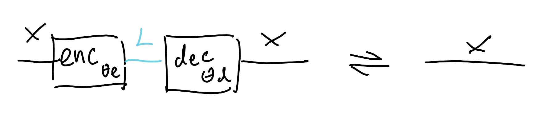
And let’s decorate the diagram a little more to recover some of the detail we squinted away. We’ll need to put in a source of data $\mathcal{X}$ that lives over the space $X$, so let’s just draw that as a state (be cool). Since we dgaf about the particular parameter spaces as we’re dealing with universal approximators, we’ll just say that enc and dec are variable functions and note down that they’re on the hook for doing something.
All the rest of the blabla is saying is: “give me a statistical divergence $\mathbf{D}$ (i.e. a spicy distance), and a bunch of data, and we want to twiddle the parameters so that the distance between left-expression applied to the data and right-expression applied to the data is small, on average.” Of course, this is needlessly complicated; the learners are just going to do whatever they can with whatever data they have to backpropagate over to make this bla-bla an equality. They want to kiss, and data+compute will help them do it. Easy-peasy; autoencoders are just an encoder and decoder tryharding to become split-idempotents, where the decoder is the retract and the encoder is the section.
Specialisations
If NNs can be anything, then we can do a directed rewrite (be cool) to make them a particular thing. The visual metaphor is we treat the variable function as a hole to plug something else into. What does that mean formally? I personally think it’s something like an operad on the homsets of an SMC (someone who actually knows category theory should check me on this).
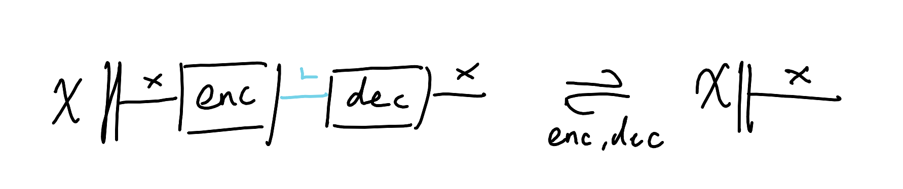
“Why is this diagram-perversion useful?” This gives us a way to compare different architectures; sometimes we can squint at a thing and see how it’s really just another thing but sparkling, or we may proactively play god and mutate things for fun and profit. Take variational autoencoders for instance. The usual presentation involves variational lower bounds, KL-divergences, and a lot of greek. But diagrammatically? It’s just a spicy autoencoder. Let’s reinvent VAEs together.
What if instead of (de/en)coding an input as deterministic points, we used probability distributions for nondeterministic (de/en)codings? We can do this in three steps: first we can make the latent space $L$ a space of (mean,variance) tuples for Gaussians:
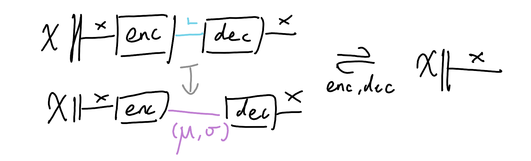
Then we can specialise the decoder to first sample from the distribution, and then decode. The whole setup still ought to behave like an autoencoder, as all we’re doing is declaring additional constraints.
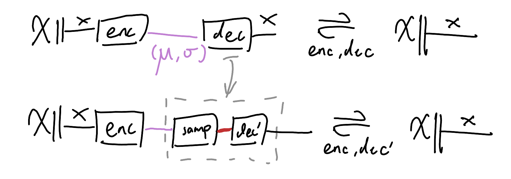
This is pretty good, now let’s re-examine our wants. We want the behaviour to be actually nondeterministic. It pays now to be paranoid: what if the encoder and decoder collude against our wishes? Maybe the encoder will always choose 0-variance encodings, so that the overall behaviour degenerates into being deterministic. Ok, so we need to strongarm the encoder into nontrivial distributions. But wait, what if the encoder still wants to cheat us by choosing means that are so far apart that the output distributions for different inputs may as well be separate points? Alright, let’s pressure the encoder to encode near the origin-centred unit-variance Gaussian then, that will sort them. We’ll add in another equational constraint.
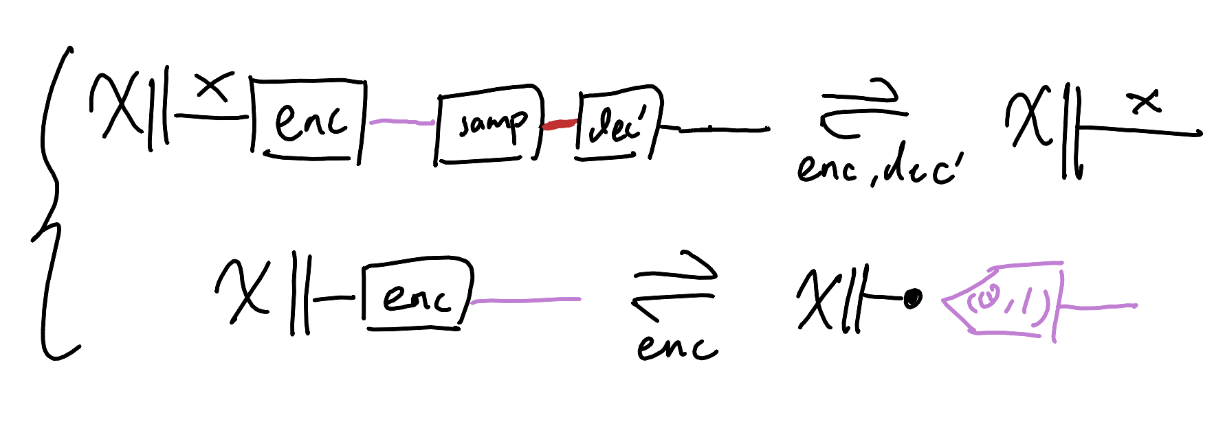
As I understand it, the term of art for such an extra rule intended to rule out unwanted behaviours is “regularisation”. Ok, kind of neat that we can in principle figure out how to regularise things with a little imagination. You know what’s extra neat? Turns out that this presentation of VAEs is equivalent to the usual very gnarly one. The consequences will leave thinkbros in shambles: we can just declare what sort of behaviours we want satisfied as equations instead of having to do math to figure it out from the ground up; we’re really embracing the idea that learners are just behaviouralist black-boxes that will do whatever they need to in order to objectivemaxx.
If this is true enough, then what would be enabling is a collection of behavioural building blocks that are already captured equationally. What kinds of behaviours do we have equations for? Good question, nephew. Let’s look at some patterns.
Patterns: Well-Understood Tasks
In this framework, we can identify certain “patterns” - common diagrammatic constraints that correspond to well-understood ML tasks. Here for example is all of supervised learning, both classification and regression:
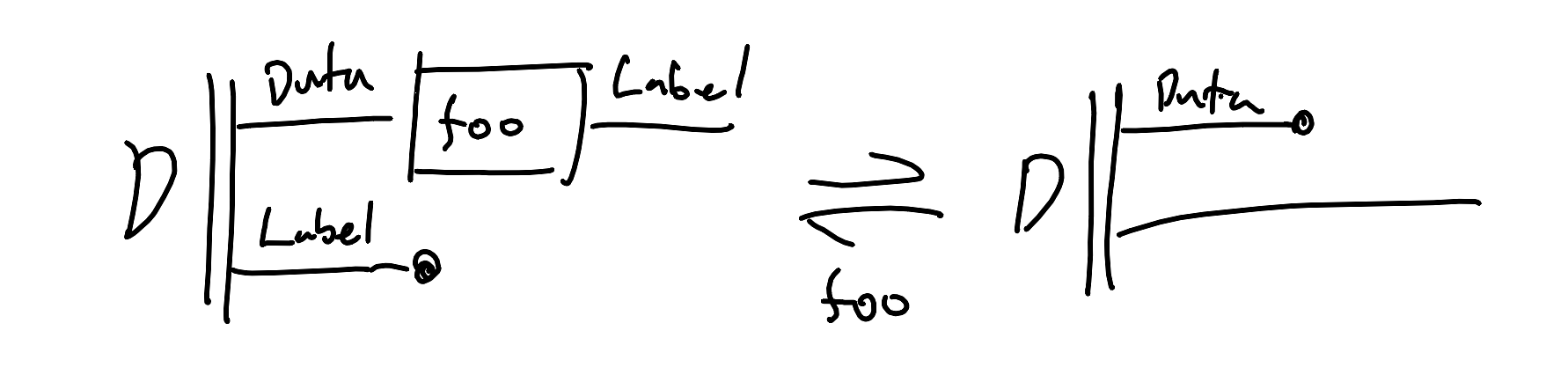
We’re solving an equation just like $1 + x = 2$, except with functions. We’re looking for a function $foo: \text{Data} \rightarrow \text{Label}$ such that for a dataset of labelled pairs $(d,l) \sim \mathcal{D}$, $foo(d) = l$. If backprop finds us such function or one that’s basically good enough, the term of art is that $foo$ is a classifier if the target labels are discrete, and $foo$ is a regressor is the target labels are continuous. From our smoothbrained perspective though, such a distinction is unnecessary.
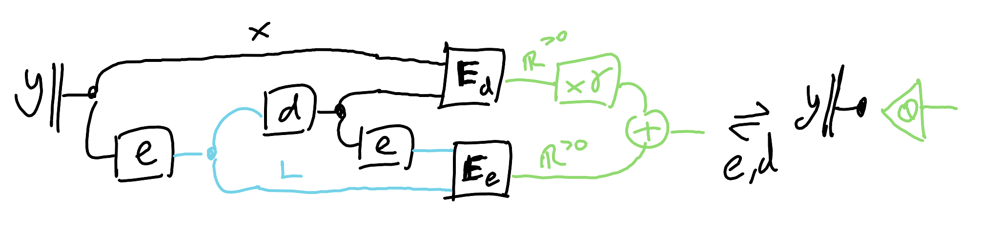
Autoencoders we’ve already done, those are good for creating representations. If you have everywhere positive measures of “energy” for representations that you want to minimise, then you get a framework to express a bunch of unsupervised learning techniques like $k$-means and PCA. Here it is as a single equation, with energy functions $\mathbf{E}_d$ and $\mathbf{E}_e$ and some positive hyperparameter $\gamma$.
Here’s a pattern I think is nice but also mysterious, and I don’t fully grok it yet. Let’s say we’re interested in generating instances of a “well-formed” subtype of a broader type, but we can’t spell out what “well-formed” means using math. For example, we might be interested in a type of “images of flowers” out of a broader type of “images”. It’s a fool’s errand to try writing out what characterises images of flowers equationally, so what else could we do? Looking at our toolkit so far, a simple option is to have a powerful classifier that recognises flowers that postselects flowers out of random images, but this is impractical, like searching the Library of Babel. We want a way for backprop to do the hard work for us of identifying what that good subspace of images is, and we can achieve this by setting up a simple dynamical system of learners. We want a generator that effectively samples the subspace of flowers, and a discriminator that distinguishes flowers from non-flowers. We want the generator produce images of flowers good enough to fool the discriminator, and we want the discriminator to pass real flowers and punish non-flowers and fake-flowers.
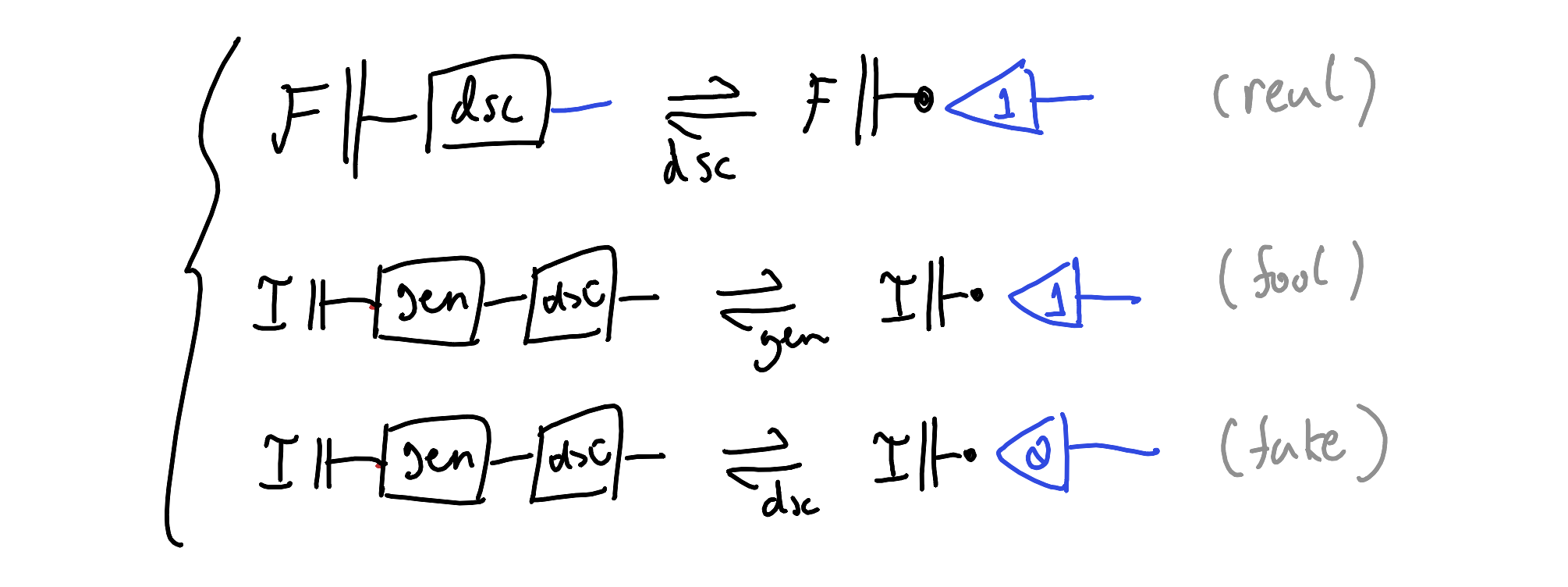
This of course is a generative adversarial network. The hope is that there is a virtuous arms-race between the generator and discriminator such that the generator produces flowers indistinguishable from the true flower-space that discriminator hones in on. The adversariality comes from the fact that by design, we cannot simultaneously have that both generator and discriminator are perfect. So we can never find a perfect representation of the GAN equations as concrete functions, and yet this unsatisfiable setup does seem to work at shrinkwrapping around otherwise ineffable subtypes. Very strange.
New Patterns?
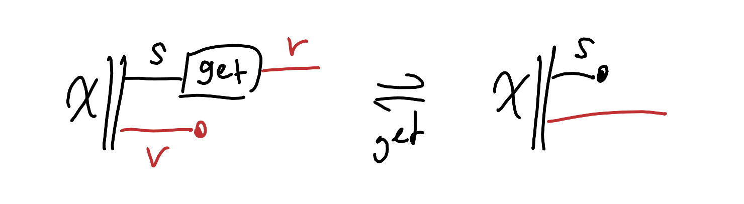
Lenses are a nice candidate from BX of a behaviour characterised in an equational, point-free way. If you’ve spent time in the bidirectional transformations crowd, you know these are just get/put pairs that obey some laws like GetPut and PutGet. If you haven’t, no worries — just know they’re a formal way of looking at and changing one attribute of a complex object while preserving the rest. So why not turn that into task-equations like we’ve already been using? If we want to manipulate attributes of data without screwing up everything else, that’s exactly what we need. Seriously, why aren’t we using these more in DL? Here’s a working recipe. We have some State data of type $S$, which carries some value data of type $V$, and we want a read-method $get: S \rightarrow V$ to look at the value of a state, and a write-method $put: S \times V \rightarrow S$ that takes a state and a new value, and returns a new state that carries the new value. First let’s ask for $get$ to behave like a classifier that learns how to extract value-features from states, trained on a labelled-dataset:
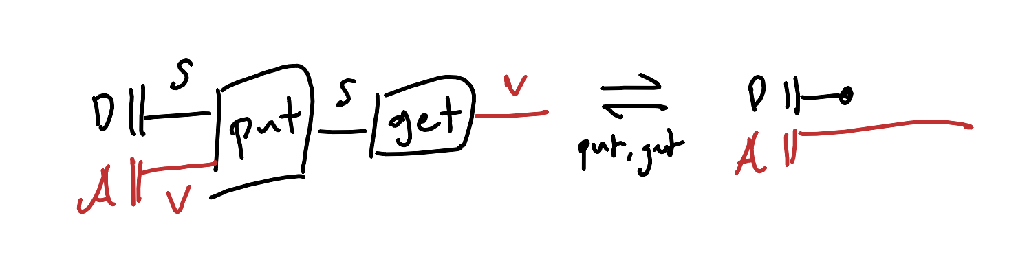
Now we want to spell out what makes the $put$ a write-method and not just some random function. It had better be the case that if we write a new value and then take a look, we can extract that new value. Let’s say that $\bar{\mathcal{X}}$ is just the state part of our data, and $\mathcal{A}$ is a random sampling of attribute values, and we’ll use these jointly independently distributed.
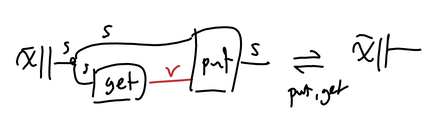
It had also better be the case that if we find that a state has a certain value, writing that same value back into the state ought to do nothing.
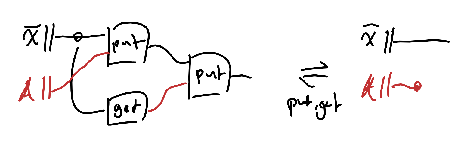
There are stronger conditions than this next one we could ask for, but we’ll just demand that we can undo changes: if we write a value in, and then change our mind and write back the old value, then we should end up with the state we started with originally.
Now, let’s say that the State is something like someone’s face, and the Value is whether that person is smiling. We want to add or remove smiles without changing other aspects like identity, hair color, or background.
TL;DR: it works. Now, a fair objection: pics or it didn’t happen.
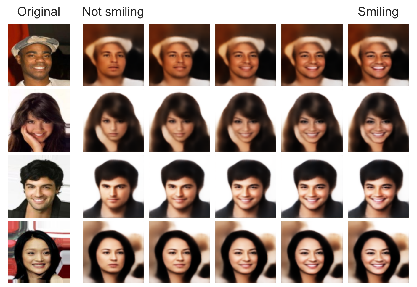
The model learns to do exactly what we want. There’s a secret extra cool thing about this example, which is that the only data the model has ever seen is faces with a binary label indicating “smile” or “no-smile”; so how is it interpolating between smiling and not-smiling? How would you do it?
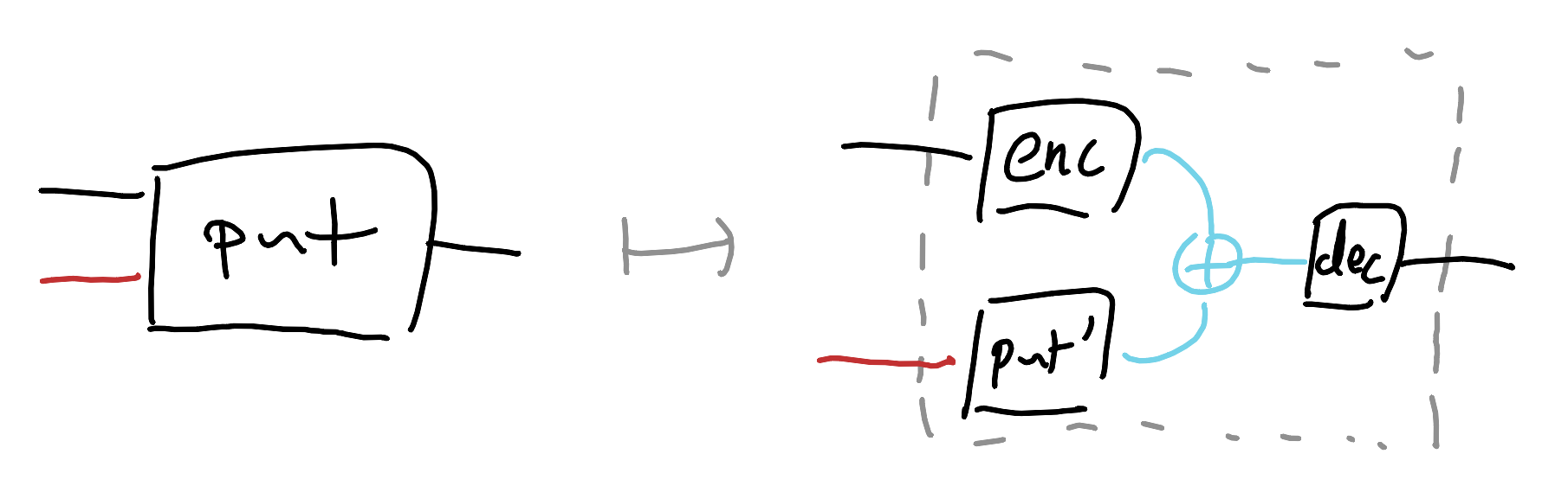
Dumber is better: if we specialise the putter to be a learned vector offset we add on to the latent of an autoencoder, then in order for the put and get to satisfy our requirements, embeddings must separate and there has to be a steering vector we can interpolate along for the different classes. No adversarial training needed, no complex masking schemes — just a task that says “change this one thing and nothing else, and make the edit a vector addition.”
Hey, here’s an idea: if you’re doing mechanistic interpretability and trying to understand things by digging in their innards, how about you stop that and just characterise what behaviours you want in a point-free way (surprise surprise that’s what category theorists are good at) and smack that DL-go-brrr. Let gradient descent figure out the implementation details. Why bother with the how when you can just declaratively specify the what?
Case Study: Computing Nash Equilibria with Gradient Descent
Check this out: I’m an idiot. I’ve been brain-damaged by string diagrams so I can’t math anymore, and also I suck at coding. My formal game theory knowledge consists of precisely two facts: Mixed Strategy Nash Equilibria exist, and they’re a pain to compute.
Have you heard the bad news? Sam Altman called, he said it’s the age of AI! You don’t have to understand phenomena in order to produce them! Verum et factum convertuntain’t, cybernetics crying in the club.
But my guy, you say, where is this going? I’m saying that I (dumbass) used string diagram objective function alchemy to bootstrap my way out of stupid and do a thing with vibe-coding, because I had the recipe for the exact behaviour I wanted drawn up with crayon ready to go.
Is this yap cap? The answer may surprise you.
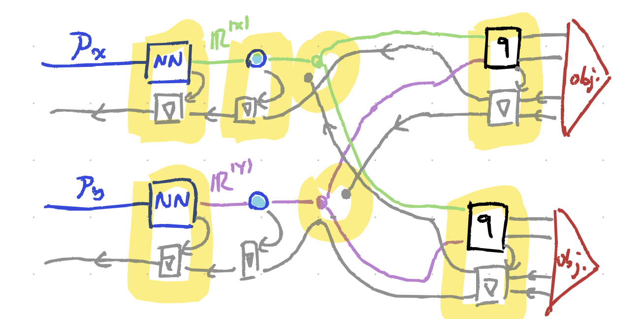
First, I sketched out a diagram for finding Mixed Strategy Nash Equilibria (MSNE) using gradient descent. If you know game theory, you’re probably thinking “that’s not novel.” True! But I didn’t need to know anything beyond “MSNE means neither player can improve by changing strategy unilaterally.”
In a 2-player game with size-$K$ finite strategy sets $X$ and $Y$, mixed strategies (i.e. probability distributions over strategies) can be viewed as points in the $K$-simplices $\Delta^{|X|}$ and $\Delta^{|Y|}$. Source: trust me bro, that’s how triangles work. So a mixed strategy for 2-players is a choice of point inside some hyperpyramid for each player. Here’s a drawing.
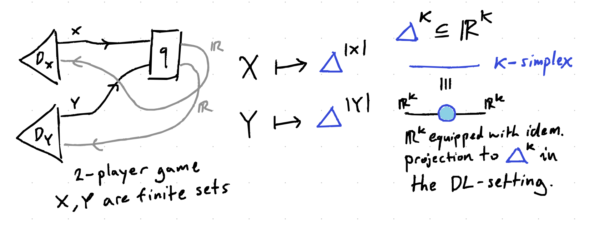
A 2-player MSNE then is a pair of points where neither player can improve their expected payoff by unilaterally changing their strategy. In other words, each player’s strategy is optimal given what the other player is doing.
🎤 Live diagrampilled reaction:
🔺 Mixed strategies are places in a triangle
🚶🏽♂️ Players are moving around in their own triangles
🚷 MSNE is when players stop moving
🤑 Stop moving = locally-payoffmaxxing
🤬 payoffmaxxing = losscels seethe
⬇️ losscels = descentcels
🤔 descentcels = downwardcels
☝️ downwardcels seethe because upwardchads
🧗🏻 upwardchads ascentmaxx
🧠 Thus ascentmaxxing = locally-payoffmaxxing
⬆️ Thus playerchads must ascend
😎 Cool fact: $\infty$ is the tallest number
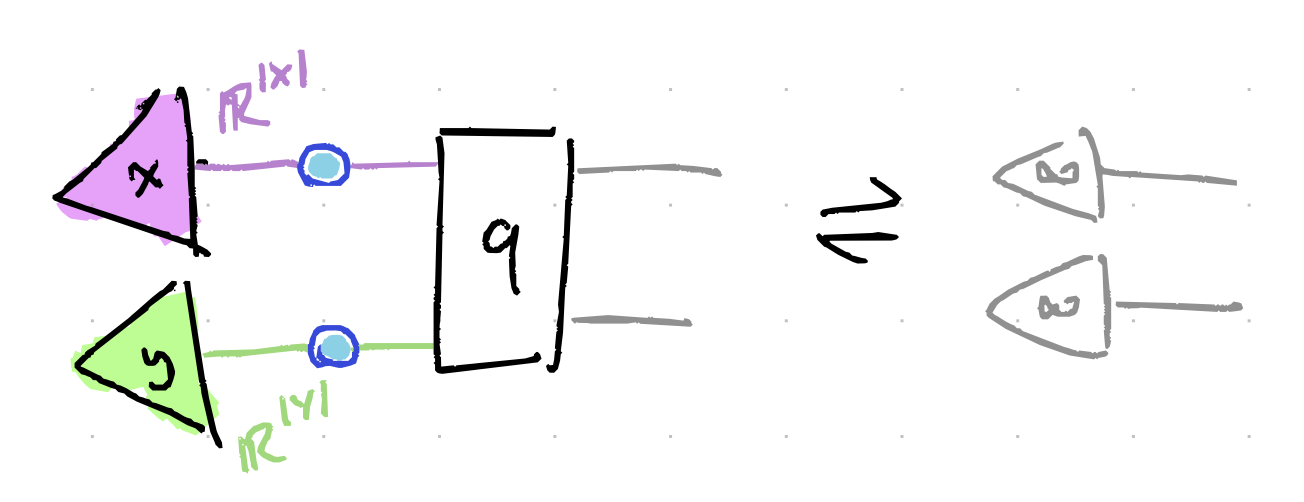
The trick is splitting the paths during backprop. Each player treats the other’s strategy as fixed when computing how to update their own strategy. This corresponds exactly to the “unilateral” part of the Nash equilibrium definition.
I showed these drawings and some words to Gemini 2.5 and asked it “make this like a computer person speak”. And then I took that and demanded “implement this and use the most DL-go-brrr”. And then I cleaned up the syntax errors in cursor by asking “😭” a few times. Tbh, the real value-add here was getting a GUI working so that it was relatively easy to change starting configurations and visualise how the strategies evolved:
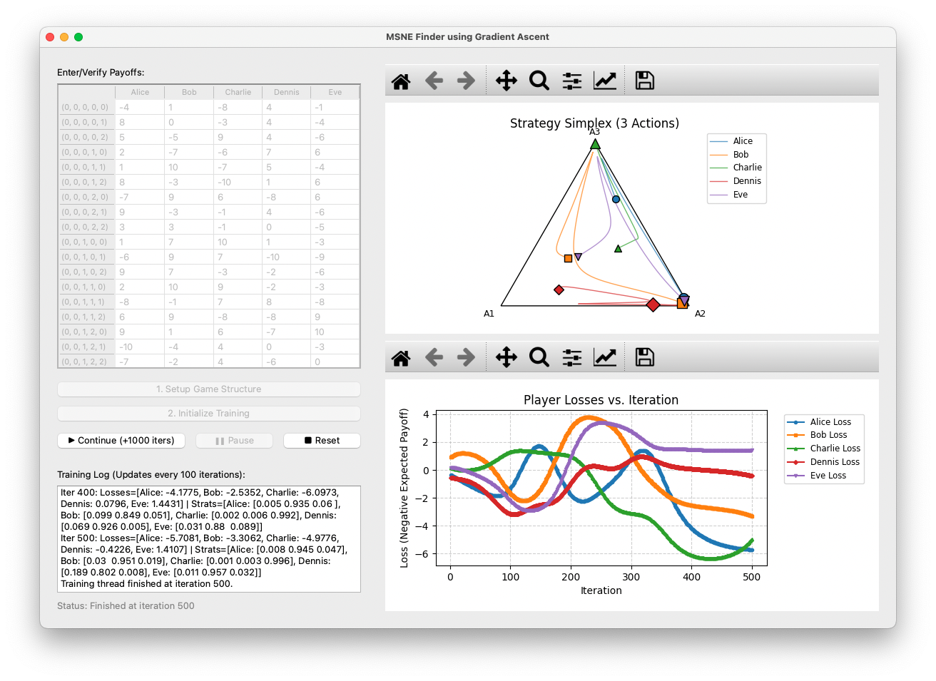
The resulting code with a more detailed math spec is all here. It works, and while this approach doesn’t scale well to more than like 7 players and 7 actions, we can always buy a new datacenter and drink another river. What’s the point of all this? It’s not that I’ve revolutionised game theory computation, it’s that I (understander of sweet fuckall) was able to direct the automatic implementation of working DL solutions just by drawing pictures and grovelling at an LLM, and that means so can you.
Conclusion
String diagrams aren’t just elegant brainrot, they’re a practical tool for cheesing deep learning. By expressing objectives as equational constraints between diagrams, we gain:
- A unified language for expressing diverse DL paradigms
- A way to build up complex objectives declaratively
- The ability to bullshit our way through domains we barely understand
The future of DL might not be about designing complex architectures, but about specifying ever more precise behaviours. You deserve a break, thinkbro: join the dark side and let the universal approximation theorem do the heavy lifting. Next time you’re designing a learning system, consider sketching its intended behaviour as a string diagram first. Or when you’re approaching a domain you know nothing about, try drawing it out diagrammatically and see if DL-powered representation theory can save you from having to learn things.