Generalized Transformers from Applicative Functors

Cross-posted on the GLAIVe blog

Transformers are a machine-learning model at the foundation of many state-of-the-art systems in modern AI, originally proposed in [arXiv:1706.03762]. In this post, we are going to build a generalization of Transformer models that can operate on (almost) arbitrary structures such as functions, graphs, probability distributions, not just matrices and vectors.

We will do this using the language of applicative functors, and indeed many of the constructions here have similar ideas to those presented in the original paper introducing applicative functors by McBride and Paterson, the only difference is that we interpret them in the context of machine learning, rather than in the context of functional programming with effects.

Although I’m not aware of this particular construction appearing elsewhere in the wild, it is related to and inspired by various other models in the literature, in particular neural operators [arXiv:2108.08481], which define models very similar to the Funcformer model that we will present later.

This work is part of a series of similar ideas exploring machine learning through abstract diagrammatical means. If you think this is interesting, I would recommend reading other posts and papers in the same series, such as:

• On the anatomy of attention [arXiv:2407.02423] (the ‘tube’ notation in Part 4 is equivalent to the ‘SIMD’ notation in that paper)
• A pattern language for machine learning tasks [arXiv:2407.02424]

These ideas were developed collaboratively in conversation with many colleagues, but in particular: Vincent Wang-Maścianica, Nikhil Khatri, Jono Liu, Ben Rodatz, Ian Fan, Neil Ortega, and Blake Wilson.

At its core, the Transformer is a method for mapping sequences of vectors to sequences of vectors. We will skip any conceptual explanation and go straight to the mathematics, since this has been explained at length elsewhere (for instance, by Grant Sanderson). We have as input a sequences of $n$ vectors $x_i \in \mathbb{R}^d$, and the model outputs a sequence $y_i \in \mathbb{R}^d$ also of length $n$. Both of these are arranged as matrices $X, Y \in \mathbb{R}^{n \times d}$. The basic operation of a Transformer relies on interleaving two different operations: multi-layer perceptrons (MLPs) and self-attention. Given learnable matrices $Q, K \in \mathbb{R}^{d \times d_k}$, $V \in \mathbb{R}^{d \times d}$, $W_1 \in \mathbb{R}^{d \times d_{ff}}$, and $W_2 \in \mathbb{R}^{d_{ff} \times d}$, and vectors $b_1 \in \mathbb{R}^{d_{ff}}$ and $b_2 \in \mathbb{R}^{d}$, these operations can be expressed as follows:

where $1_n \in \mathbb{R}^n$ is the all-ones vector, $\sigma : \mathbb{R} \to \mathbb{R}$ is an activation function applied element-wise that is usually taken as $\sigma(x) = \mathrm{ReLU}(x) = \max(x, 0)$, and $\rho : \mathbb{R}^n \to \mathbb{R}^n$ is a normalization function applied to each column that is usually taken as the scaled softmax:

A (single-headed) Transformer can be built by iterating these functions (each with separate learnable weights) along with some other components like residuals and layer-norms that we will omit here for simplicity.

Part 1: A basic model

Suppose we wanted to implement a machine-learning model like the Transformer in a functional programming language - in this post we will use Haskell. We can start with a very naive type-level model, taking vectors as lists and matrices as lists of row-vectors. It is easy to build up the basic components like dot products, vector-matrix multiplication, and matrix-vector multiplication:

-- Dot product of two vectors
dot :: [Float] -> [Float] -> Float
dot a b = sum $ zipWith (*) a b

-- Multiply a matrix by a vector from the right
mulMV :: [[Float]] -> [Float] -> [Float]
mulMV m v = map (`dot` v) m

-- Sum a list of vectors
vectorSum :: [[Float]] -> [Float]
vectorSum = foldl (zipWith (+)) (repeat 0.0)

-- Multiply a matrix by a vector from the left
mulVM :: [Float] -> [[Float]] -> [Float]
mulVM v m = vectorSum $ zipWith (map . (*)) v m 

-- Multiply a matrix by another matrix
mulMM :: [[Float]] -> [[Float]] -> [[Float]]
mulMM a b = map (`mulVM` b) a

-- Multiply a matrix by the transpose of another matrix
mulMMT :: [[Float]] -> [[Float]] -> [[Float]]
mulMMT a b = map (a `mulMV`) b

And from here we can build the MLP and self-attention operations. In this case we build self-attention from a generic attention operation, where $XQ$, $XK$, and $XV$ are provided directly:

scaleSoftmax :: Int -> [Float] -> [Float]
scaleSoftmax dk v = map (/ n) e 
    where e = map exp v
          n = sqrt (fromIntegral dk) * sum e

-- A generic attention function, before the inputs are specialized
attention :: [[Float]] -> [[Float]] -> [[Float]] -> [[Float]]
attention queries keys values = attMatrix `mulMM` values
    where dk = length $ head queries
          -- The 'attention matrix'
          attMatrix = map (scaleSoftmax dk) (queries `mulMMT` keys)

selfAttention :: [[Float]] -> [[Float]] -> [[Float]] -> [[Float]] -> [[Float]]
selfAttention Q K V X = attention (X `mulMM` Q) (X `mulMM` Q) (X `mulMM` V)

-- Apply a linear function f(X) = XW^T + 1b^T to the input
linear :: [[Float]] -> [Float] -> [[Float]] -> [[Float]]
linear weights bias input = map (zipWith (+) bias) (input `mulMMT` weights)

mlp :: [[Float]] -> [Float] -> [[Float]] -> [Float] -> [[Float]] -> [[Float]]
mlp W1 b1 W2 b2 X = linear W2 b2 $ map (map relu) $ linear W1 b1 X
    where relu x = max 0.0 x

There are two major problems with this code:

1. Since the dimensions of the problem are not encoded in the types, it would be easy to pass a malformed input to these functions. For example, accidentally transposing the weights of an MLP would neither be caught at compile-time nor result in a runtime error.
2. It would seem this code is too specific - all these operations ought to be possible over more generic structures than just [[Float]], wouldn’t it be better if the code could handle any appropriate structure?

Part 2: Fixing the problems

We will solve both of these at the same time. As a first guess, since the list type is a monad, is it it possible to generalize this code to any monad? The components we would need are:

map :: (a -> b) -> [a] -> [b]
zipWith :: (a -> b -> c) -> [a] -> [b] -> [c]
vectorSum :: [[Float]] -> [Float]
sum :: [Float] -> Float

This initially looks promising, since we could substitute the first three with

fmap :: Functor f => (a -> b) -> f a -> f b

liftM2 :: Monad m => (a -> b -> c) -> m a -> m b -> m c
liftM2 f xs ys = do
    x <- xs
    y <- ys
    return $ f x y

join :: Monad m => m (m a) -> m a
join = (>>= id)

and the type signatures would match! However, substituting the list monad into these functions gives the wrong answer - while fmap is correct, liftM2 and join behave like cartesian products rather than like zips:

liftM2 (,) [1, 2] [1, 2] = [(1, 1), (1, 2), (2, 1), (2, 2)] 
                        != [(1, 1), (2, 2)] 
                         = zip [1, 2] [1, 2]
join [[1, 2], [1, 2]] = [1, 2, 1, 2]

Indeed, this is also related to our first problem. To solve that, let’s assume that the dimension of each vector was encoded in its type as Vector N a where N is a type-level natural number. As before, we will take matrices to be vectors of vectors. In this setting, no function that has this cartesian-product behaviour could exist, because the length of the vector would not be preserved, so it would not type-check. It seems even that Vector N cannot be a monad in a non-trivial way, because any join-like function would have to ‘throw away some information’ in general: since there are no non-trivial generic functions a -> a -> a, then given $N^2$ values of a generic type a that we must compress to only $N$ values, we have to discard almost all of them.

For the same reasons, such a generic version of vectorSum or sum that applies to any interior type a is too generic - we would end up throwing away information. The solution for this is to just abstract over these definitions. Let’s define a class that encapsulates these operations:

class Counit f a where
    counit :: f a -> a

So for instance we would have Monad m => Counit m (m a) given by join, and for comonads we could have Comonad m => Counit m a given by extract. In this way, we don’t have to define Counit generically, but only for types a which have a meaningful and non-trivial counit operation.

To solve the problem with liftM2, we can be careful to define Vector N so that fmap behaves the same as map and liftM2 does behave the same as zipWith. However, as we determined, Vector N shouldn’t be a monad. But it can be an applicative functor! Indeed, liftM2 is the monad specialization of liftA2:

liftA2 :: Applicative f => (a -> b -> c) -> f a -> f b -> f c
liftA2 f a b = (fmap f a) <*> b

Applicative functors are a superset of monads that are defined by the Applicative class. It is usually defined by a pair of functions

pure :: Applicative f => a -> f a
f <*> a :: Applicative f => f (a -> b) -> f a -> f b

where if we think of applicative functors as collections, pure can be interpreted as a ‘unit’ mapping any value into a collection, and <*> can be interpreted as taking a collection of functions and a collection of arguments and returning a collection of results. However, there is a more concrete definition in terms of pair:

pair :: Applicative f => f a -> f b -> f (a, b)

which can be thought of as pairing up elements of collections. These definitions are equivalent, since we have:

pair a b = (fmap (,) a) <*> b
f <*> a = fmap (uncurry ($)) $ pair f a 

We will work in terms of pair, since this is closer to the category-theoretic definition of an applicative functor as a ‘monoidal functor with tensorial strength’.

With this in mind, we can define (ignoring some Haskell specifics regarding type-level naturals)

data Vector (N :: Natural) a = Vector [a] 

instance Functor (Vector N a) where
    fmap f (Vector xs) = Vector $ map f xs

instance Applicative (Vector N a) where
    pure a = Vector $ take N $ repeat a
    pair (Vector a) (Vector b) = Vector $ zip a b

and we can see that now pair matches exactly with zip, as we wanted! See page 4 of McBride and Paterson for a similar construction.

Part 3: Applicative matrix operations

To recreate our original code in these new terms, we are still missing a few elements specific to Floats that we don’t have in the generic picture. We will ignore the scaled-softmax and ReLU operations for now as they can in principle be replaced with any normalization and activation functions, and come back to them later. However, we still need a definitions of multiplication and addition. We will just abstract over these as a typeclass:

class Ring a where
    zero :: a
    (~+~) :: a -> a -> a
    (~*~) :: a -> a -> a

We can then recover our definitions of sum and vectorSum in terms of Vector N by constructing the appropriate Counit instances:

instance Ring a => Counit (Vector N) a where
    counit (Vector xs) = foldl (~+~) zero xs

instance (Ring a, Applicative f) => Counit (Vector N) (f a) where
    counit (Vector xs) = foldl ((.) (fmap $ uncurry (~+~)) . pair) (pure zero) xs

With these definitions, we can build a fully generic version of our code that also encode dimensionality information in the type-signatures. We need only operations from the typeclasses we’ve defined, and substituting in Vector as our functor will yield something equivalent to our original code, and hence the original Transformer!

The matrix operations can be given as:

dot :: (Applicative f, Ring a, Counit f a) => f a -> f a -> a
dot a b = counit $ uncurry (~*~) <$> pair a b

mulMV :: (Applicative f, Applicative g, Ring a, Counit g a) => f (g a) -> g a -> f a
mulMV m v = uncurry dot <$> pair m (pure v) 

mulVM :: (Applicative f, Applicative g, Ring a, Counit f (g a)) => f a -> f (g a) -> g a
mulVM v m = counit $ fmap (uncurry (~*~)) . uncurry pair <$> pair (pure <$> v) m

mulMMT :: (
    Functor h, Applicative f, Applicative g, Ring a, Counit g a
) => f (g a) -> h (g a) -> h (f a)
mulMMT = fmap . mulMV

mulMM :: (
    Applicative h, Functor f, Applicative g, Ring a, Counit g (h a)
) => f (g a) -> g (h a) -> f (h a)
mulMM = flip $ fmap . flip mulVM

So we see that instead of defining a matrix as [[Float]] and a vector as [Float], these have become f (g a) and f a respectively for arbitrary type constructors f and g and arbitrary ‘scalar’ types a. If f and g are different instances of Vector N for example, then this will prevent many bugs of the type we identified earlier with stronger compile-time checks.

By abstracting over the scaled-softmax and ReLU functions as arbitrary functions that can be passed in, we can define the generic attention and linear function operations as before:

attention :: (
    Applicative f, Applicative g, Ring a, Counit g a, Counit f (g a)
) => (f a -> f a) -> f (g a) -> f (g a) -> f (g a) -> f (g a)
attention softmax queries keys values = attMatrix `mulMM` values
    where attMatrix = fmap softmax (queries `mulMMT` keys)

linear :: (
    Applicative g1, Applicative g2, Ring a, Counit g1 a
) => g2 (g1 a) -> g2 a -> g1 a -> g2 a
linear weights bias input = fmap (uncurry (~+~)) $ pair bias $ mulMV weights input

And we can put it all together to define self-attention and MLP operations. We can make it a bit nicer than before by packaging all the matrices together as data-structures:

data SelfAttention s d a = SelfAttention {
    -- This abstracts scaled-softmax
    softmax :: s a -> s a,
    queryMat :: d (d a),
    keyMat :: d (d a),
    valueMat :: d (d a)
}

runSelfAttention :: (
    Ring a, Applicative s, Applicative d, Counit d a, Counit s (d a)
) => SelfAttention s d a -> s (d a) -> s (d a)
runSelfAttention SelfAttention { softmax, queryMat, keyMat, valueMat } input = 
    attention softmax queries keys values
    where queries = mulMMT queryMat input
          keys = mulMMT keyMat input
          values = mulMMT valueMat input

data MLP din dff dout a = MLP {
    -- This abstracts ReLU
    activation :: a -> a,
    weights1 :: dff (din a),
    bias1 :: dff a,
    weights2 :: dout (dff a),
    bias2 :: dout a
}

runMLP :: (
    Ring a, Applicative dff, Applicative dout, 
    Counit dff a, Applicative din, Counit din a
) => MLP din dff dout a -> din a -> dout a
runMLP MLP { weights1, bias1, weights2, bias2, activation } = 
    linear weights2 bias2 . fmap activation . linear weights1 bias1

Finally, we can combine these blocks to make a whole Transformer. We are ignoring the layer-norms, and using only a single attention head, but otherwise this is identical to the original proposal from Vaswani et al:

-- One transformer layer is a self-attention block and an MLP block with residuals
data TransformerLayer s d dff a = TransformerLayer {
    mlp :: MLP d dff d a,
    satt :: SelfAttention s d a
}

runTransformerLayer :: (
    Ring b, Applicative dff, Applicative d, Applicative s, 
    Counit dff b, Counit d b, Counit s (d b)
) => TransformerLayer s d dff b -> s (d b) -> s (d b)
runTransformerLayer TransformerLayer { mlp, satt } = 
    residual (runMLP mlp <$>) . residual (runSelfAttention satt)
    where add x y = fmap (uncurry (~+~)) . uncurry pair <$> pair x y
          residual f x = add (f x) x 

-- A transformer is a linear embedding matrix, followed by a 
-- stack of transformer layers composed sequentially, 
-- followed by a linear unembedding matrix
data Transformer s f d dff a = Transformer {
    layers :: [TransformerLayer s d dff a],
    embed :: d (f a),
    unembed :: f (d a)
}

runTransformer :: (
    Ring a, Applicative f, Applicative d, Applicative dff, Applicative s, 
    Counit d a, Counit dff a, Counit s (d a), Counit f a
) => Transformer s f d dff a -> s (f a) -> s (f a)
runTransformer Transformer { layers, embed, unembed } = 
    mulMMT unembed 
    . flip (foldl (flip runTransformerLayer)) layers 
    . mulMMT embed

Part 4: Diagrammatics

(Many thanks to Vincent Wang-Maścianica for his help with this part)

All this uncurrying we needed to do to write the code above using pair is pretty miserable. That’s because we are trying to do fundamentally 2D things in 1D and it sucks. Luckily there is a formal diagram system for this.

We build on the tube-notation for monoidal monads introduced by Joe Moeller in his blogpost, which is an evident extension of functor box notation, by stretching out functor-boxes as “windows” along the length of wires to become “tubes”. So if we have an underlying symmetric monoidal category $(\mathcal{C},\otimes,I)$ along with a symmetric monoidal endofunctor $\mathbf{T}: \mathcal{C} \rightarrow \mathcal{C}$, we would depict the object $\mathbf{T}X$ of $\mathcal{C}$ as the wire $X$ wrapped by a $\mathbf{T}$-tube:

As is sort-of known, applicative functors are equivalently lax-monoidal functors with a tensorial strength. In tube-notation, the laxator natural transformation $\tau_{-,=} : \mathbf{T}(-) \otimes \mathbf{T}(=) \rightarrow \mathbf{T}(- \ \otimes =)$ are depicted as pants that merge two parallel tubes:

This is exactly the pair operation we have in the code above. The visual tube metaphor captures the naturality conditions we want string-diagrammatically, as deformation of string diagrams freely within the confines of tubes. For example, this pretty little monster is the naturality condition that allows the laxator to cohere with a simplified form of interchange, given two morphisms $f: A \rightarrow X$ and $g: B \rightarrow Y$:

But all we’re really asking for here in string-diagrammatic terms is that you can slide morphisms around in pants that merge tubes.

The rest of the lax monoidal structure goes as one would expect. For example, we want the monoidal laxator to be appropriately associative (we won’t label wires with types anymore, they can be any object in the category.)

There’s also another laxator $\nu: I \rightarrow \mathbf{T}I$ for the monoidal unit (depicted here with a dashed wire)

And these laxators should behave as we expect, namely they should be appropriately unital. Below we get the middle equalities (depicting the left and right unitor isomorphisms of $\mathcal{C}$) for free, as we can assume that we’re working with a strict symmetric monoidal category.

And of course, we would like the laxators to cohere sensibly with braidings.

Now the tensorial-strength, which is a natural transformation $\beta: - \otimes \mathbf{T}(=) \rightarrow \mathbf{T}(- \ \otimes =)$. In tube-notation, this corresponds to taking a wire and shoving it inside an adjacent tube.

There are a couple of coherence conditions we expect, namely that it doesn’t matter whether we shove wires in one-by-one or all at once, that shoving-in the monoidal unit does nothing, and that shoving-in can be done from either side in a way that coheres with the braiding.

And we’re done with the tricky bit. In terms of the code above, this is

beta :: Applicative f => a -> f b -> f (a, b)
beta a b = pair (pure a) b

nu :: Applicative f => () -> f ()
nu () = pure ()

which along with $\tau$ (equivalently pair) and the right unitor $\rho$ from above is also enough to define pure:

rho :: Applicative f => f (a, ()) -> f a
rho = fmap fst

pure :: Applicative f => a -> f a
pure a = rho $ beta a $ nu ()

completing the equivalence between the diagrams and the code.

The other ingredients we need are garden-varietal diagrammatic gadgets. We will need a copy-gadget, which we can have in any Cartesian (or Markov) category. Copy comonoids are traditionally depicted as dots that gather the various copied branches. Since we will be copying tubes, which will make dots too big, we will use a fork-notation for copying instead.

We will need learnable parameters, such as weights and biases. These are just elements of a given object (for instance, $\mathbf{TT}X$ or $\mathbf{T}X$) and to be depicted as triangles, though to indicate that it is a learner with some parameter space, for historical reasons ¹ we will colour them red.

We will need an algebra $\alpha_X \mathbf{T}X \rightarrow X$ (this is Counit) which extracts wires from tubes. We’ll depict these as triangles that cap off tubes.

We will need some magma $X \otimes X \rightarrow X$ (this is ~*~ from Ring). In practice, the multiplication of any off-the-shelf monoid will do.

Optionally, we may have a “normalisation” $\sigma: \mathbf{TT}X \rightarrow \mathbf{TT}X$ (which generalizes softmax).

Now we can assemble these ingredients. The pants, magma, and the algebra allow us to define an abstract inner product of type $\mathbf{T}X \otimes \mathbf{T}X \rightarrow X$.

We can also define an abstract outer product of type $\mathbf{T}X \otimes \mathbf{T}X \rightarrow \mathbf{T}\mathbf{T}X$, using the magma and two instances of the tensorial strength of the applicative.

Now we’re ready for the abstract attention mechanism. The idea is to use the outer product gadget to create a doubly-nested tube, and then to use the inner product gadget along with the pants and shoving of the applicative to bring that back down to a singly-nested tube, while liberally sprinkling in learners. Since the outer product requires two $\mathbf{T}X$ inputs, and we require at least one extra copy of $\mathbf{T}X$ apart from those to use the inner product, it makes sense to start with three copies of the initial input $\mathbf{T}X$, and a little thought will yield this:

For the sake of convention, we put learnable linear transformations on the three inputs and call them “queries”, “keys”, and “values”. This is exactly the same as runSelfAttention. If we pick $X$ to be $\mathbb{R}$, our applicative functor to be the $k$-tupling endofunctor $X \mapsto X^k$, where $k$ is some positive integer “context-length” for the outer tubes and a “model dimension” for the inner tubes, and if we choose our algebra to be summation, our monoid to be multiplication, and our normalisation to be softmax, then we have precisely a classic attention mechanism as in the matrix-based selfAttention above. The $\mathbf{TT}X$ wire in this case is the abstract analog of the attention matrix; the synthetic inner and outer products we define here are special cases of tensor contraction, where each index of a tensor corresponds to a layer of tubing.

Part 5: Funcformer

At this point, we are done in theory! We have a fully generalized construction of a Transformer model. However, what does this buy us in practice? Can we construct anything meaningfully different than the standard model? Indeed there is, and we shall look at one such construction now, which we call Funcformer. We start with this not necessarily because it is the most useful generalization we can make, but because it is the easiest to implement.

One potential generalization of the Vector N type comes from viewing any vector $v \in X^{n}$ over some type $X$ as a function from indices to components of the vector - i.e $v : {1, 2, \dots, n} \to X$ given by $v(i) = v_i$. There is no fundamental reason why this index set ought to be finite, or even discrete. To that end, let’s define a ‘continuous vector’ CVector which has ‘components’ parameterized by a real number. We can define this in code as

newtype CVector a = CVector { (~!!~) :: Float -> a }

where the ~!!~ operator is analogous to the indexing operator on lists, !! : [a] -> Int -> a. This type is indeed an applicative functor (in fact, it is a specialization of the Reader monad):

instance Functor CVector where
    fmap f x = CVector { (~!!~) = f . (x ~!!~) } 

instance Applicative CVector where
    pure x = CVector { (~!!~) = const x }
    pair x y = CVector { (~!!~) = \t -> (x ~!!~ t, y ~!!~ t) }

Mathematically, we can think of v : CVector a as a function $v \in \mathbb{R} \to a$, and we will notate it as such (i.e $v(x)$). Then the operations defined here can be interpreted as

We also need instances of Counit for this type. Here, we can draw some inspiration from the original Transformer, where these corresponded to sums over the components of vectors, or sums of the rows of a matrix. Analagous to a sum over a vector, we can consider the integral of a function over its domain - of course, this is not straightforward to define in code, but let’s pretend we have a magical black box:

integrate :: (Float -> Float) -> Float

Using this we can define:

instance Counit CVector Float where
    counit f = integrate (f ~!!~)

instance Counit CVector (CVector Float) where
    counit f = CVector { (~!!~) = \y -> integrate (\x -> f ~!!~ x ~!!~ y) }

Note here that our equivalent of a matrix, v : CVector (CVector a) is equivalent to a function with type $v : \mathbb{R} \to \mathbb{R} \to a$. By currying, this is the same as a two-argument function $v : \mathbb{R}^2 \to a$, and so we will notate it as $v(x, y)$. We can again interpret these operations mathematically, as:

This is actually all we need to translate the whole Transformer into CVectors! Working through the code, we can have a look at what the building blocks operations become, mathematically:

It is pleasing to see that dot products over vectors translate directly into the $L^2$ dot product on functions, and that the multiplication operations generalize matrix multiplication exactly as one would expect! (I’ve skipped the transposed versions here because they are symmetric.) Given $Q, K, V, W_1, W_2 \in \mathbb{R}^2 \to \mathbb{R}$, and $b_1, b_2 \in \mathbb{R} \to \mathbb{R}$, the MLP operation becomes

where $\sigma \in \mathbb{R} \to \mathbb{R}$ is some arbitrary activation function. If we take the obvious continuous generalization of the scaled-softmax operator to be given by

then we can write the self-attention operation as:

This is pretty gnarly! Obviously, there are very few functions where you could expect this to be exactly solvable, and really I’m only writing it down here to show that it does in fact exist.

To regroup, let’s just remind ourselves what we just derived: we replaced Vectors in the original Transformer with CVectors and so now we have a model that instead of mapping matrices to matrices, maps two-argument functions to two-argument functions! In the usual interpretation of the Transformer as it is applied to natural language processing, we consider one dimension of the matrix to be the ‘sequence’ dimension (that is, it represents your position in the text), and the other to be the ‘feature’ dimension (that is, it represents something about the meaning of the words at each position). So in our model, we can think perhaps that we have a continuum of text positions, and a continuum of features at each position, rather than finitely many of each.

So how can we make this idea practical? We need a way to represent functions and integration efficiently, and hence in a finite-dimensional way. This could be done with a table of values for each function and numerical integration, but it’s both more efficient and more interesting to choose a different method. Since any function can be approximated as a polynomial, and it is easy to integrate polynomials, we can choose a set of polynomials that is closed under addition as our finite-dimensional representation. In particular, we make the following (arbitrary) choice, representing functions as 1D or 2D Chebyshev series:

where $T_n(x)$ represents the $n$-th Chebyshev polynomial of the first kind. Moreover, rather than considering domain of our functions to be the whole real line, we will just consider the range $[-1, 1]$. This choice of polynomials has the advantage that it is more numerically stable when interpolating data points than the standard monomial $a + bx + cx^2 + \cdots$ basis.

For $n, m, |n - m| \geq 1$ (and the other cases follow similarly), we can use a known result about Chebyshev polynmomials, that

which we define to be the components of the weight matrix $W_{n, m}$. Suppose then that we have two functions $f(x)$ and $g(x)$ represented as series with coefficients $f_i$ and $g_i$, then we can write their dot product defined above as

if $f_* $ and $g_* $ are vectors representing the coefficients of the series. So we can see that a dot product of functions has become simply a dot product of vectors, albeit with respect to a different bilinear form than the usual dot product!

Indeed, this is also true for the (abstract) matrix-vector and matrix-matrix multiplication operations defined above. In the same way as above, let us denote $m_*$ as the matrix of coefficients $m_{ij}$ corresponding to a two-argument function $m(x, y)$. We have that:

This is almost all the parts we need to build a Transformer. The only thing that is left is activation function for the MLP and the softmax operation. While in the applicative-based code above, these were specified as element-wise and ‘row’-wise operations, respectively, in practice they could be almost anything.

For the activation function, we chose to keep very close to the original definition - you can approximately apply an elementwise operation to a function represented as a Chebyshev series by first evaluating the polynomial on a grid of points, applying the operation to each of those points, and then interpolating a series from the new values. This is particularly efficient for Chebyshev polynomials, as transforming between the series and point-grid representations can be done using a variant of the fast Fourier transform called the discrete Chebyshev transform, see for instance here for details. We used this technique to apply the ReLU activation function.

For the softmax, we chose a slightly less faithful implementation, by applying the softmax operation row-wise directly to the matrix of coefficients. This is much more efficient than trying to apply it to the function values themselves, and seems to work well in practice. We note that the original purpose of the softmax in the Transformer is to ensure that each row of the ‘attention matrix’ $XQ(XK)^T$ has nicely bounded values, and in the continuous case this is also achieved by applying the softmax to a coefficient vector, since bounded coefficients imply a bounded value of the overall function in a given domain.

At this point it is worth noting that this model is very similar to those constructed in the literature of neural operators [arXiv:2108.08481] [arXiv:2003.03485]. In particular a model called the Fourier neural operator [arXiv:2010.08895] is a quite similar idea, replacing Chebyshev series with Fourier series. It is a good sanity check to see that our generic approach has yielded a model that has been previously considered and is regarded to be useful in practice, and it suggests that continuing this line of thought may lead to more useful models!

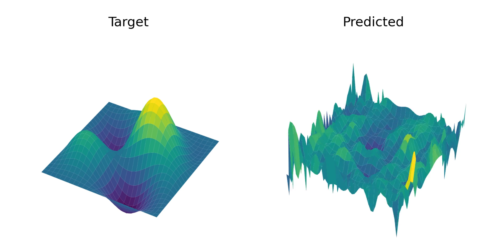
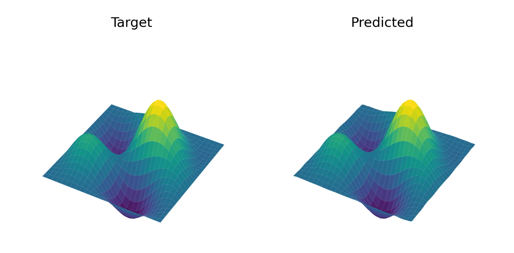
With these details worked out, it is possible to build this model explicitly in a machine learning framework such as PyTorch - we have a very basic implementation available on GitHub. As a very simple test, we can try the following task - given a function $f(x, y)$ we can define Poisson’s equation:

This is a partial differential equation that can be solved numerically via a variety of strategies (for instance, finite difference or collocation approaches). The right hand side $f(x, y)$ is conventionally known as the ‘source term’, and the solution $g(x, y)$ is sometimes called the ‘potential’. Since the process of solving this equation can be thought of as a map from source term to potential, then rather than solving this equation numerically, we will train a Funcformer model to do it for us! Note that this is not training a model to approximate the solution to a particular instance of Poisson’s equation but a more general map from source terms to potential, as in the theory of operator learning [arXiv:1910.03193].

We trained the model on random smooth functions (i.e the highest-order Chebyshev coefficients were fixed to zero) with fixed boundary conditions of $f(x, \pm 1) = f(\pm 1, y) = 0$, and it appears to converge well. See below for an example solution, and see YouTube for a video of how this example evolves throughout training.

Part 6: A generalized Transformer zoo

However, CVector is not the only alternative applicative functor we could use - let’s run through some more that might be interesting! Before we start, it’s worth pointing out that while we are using functional programming as a way to express these ideas, in practice these models can and should be implemented in an imperative language using a machine learning framework, as for any other model.

Expression trees and DAGs

Suppose we have a binary tree datatype defined like

data Tree l = Node (Tree l) (Tree l) | Leaf l

then this is indeed an applicative functor:

instance Functor Tree where
    fmap f (Node left right) = Node (fmap f left) (fmap f right)
    fmap f (Leaf x) = Leaf $ f x

instance Applicative (Tree op) where
    pure x = Leaf x
    pair (Node la ra) (Node lb rb) = Node (pair la lb) (pair ra rb)
    pair (Node l r) (Leaf x) = Node (fmap (,x) l) (fmap (,x) r)
    pair (Leaf x) (Node l r) = Node (fmap (x,) l) (fmap (x,) r)
    pair (Leaf x) (Leaf y) = Leaf (x, y)

We can think of the pair operation here as mapping two trees to their common refinement (i.e the smallest tree containing them both) by expanding leaves to subtrees where necessary, and then zipping the two trees together. Given any method of combining two leaves (for example, addition), we can define a counit for trees by combining leaves from the bottom-up:

instance Ring a => Counit Tree a where
    counit (Node l r) = counit l ~+~ counit r
    counit (Leaf x) = x

instance (Ring a, Applicative f) => Counit Tree (f a) where
    counit (Node l r) = uncurry (~+~) <$> pair (counit l) (counit r)
    counit (Leaf x) = x

We have previously tried to implement this in practice, but as you would expect it is very hard to do efficiently and especially in a GPU-accelerated way!

It is important to note that with this definition, all the structure of the trees has to be present in the input data, in some form - the generalized Transformer model cannot be used to, for example, infer a tree structure from data (at least not directly), because the output tree will always be the common refinement of the inputs - what the model is learning to modify is the values of the leaves.

There are two obvious extensions to this: general expression trees, where the operations used to combine each node may be stored in the node itself, and directed-acylic graphs, where the node combination procedes from sources to sinks. Various applications of this come to mind, for example, code synthesis and comprehension, or structured data retrieval.

Probability distributions

It is well known that you can form a monad from probability distributions (indeed, finite discrete distributions are essentially a variant of the list monad discussed earlier), and since all monads are applicative functors, this is sufficient for our purposes. We can write

data Distribution a = Distribution [(a, Float)]

to represent a finite discrete distribution, and we assume that it is constrained so that the probabilities can only take positive values, and sum to one. This is indeed a functor as expected:

instance Functor Distribution where
    fmap f (Distribution dist) = Distribution $ map (\(x, p) -> (f x, p))

instance Applicative Distribution where
    pure x = Distribution [(x, 1.0)]
    pair (Distribution a) (Distribution b) = 
        Distribution $ zipWith (\(x, px) (y, py) -> ((x, y), px * py)) a b

This would be very inefficient, and in practice, you should perform some kind step to combine equal outcomes in the distribution (but this is not permitted by the type signature of Applicative since it would require an equality typeclass constraint or similar). Indeed, this restriction is only due to the confines of expressing these operations in Haskell (where all functors must be endofunctors on $\mathrm{Hask}$), certainly continuous probability distributions also form a monad, and thus an applicative functor. For instance, if $X \sim D$ is a random variable, then the random variable $f(X) \sim f(D)$ should be well-defined if the codomain of $f$ is measurable. We would like to write this

data Distribution a = Distribution { pdf :: a -> Float }

instance Functor Distribution where
    fmap f dist = Distribution { pdf = ... }

but it is not possible to implement Functor here in a sensible way. This is possible with more advanced types, see for instance the monad-bayes package. Counit could be defined in many ways, but taking the expectation value of the distribution would appear to be a somewhat canonical choice:

instance Counit Distribution Float where
    counit (Distribution dist) = sum $ map (uncurry (*)) dist

To make this practical, we could imagine parameterizing the space of all probability distributions either with finite discrete distributions as we defined above, or by some finite-dimensional representation such as a mixture of Gaussians. Furthermore, probability distributions over probability distributions (in the sense of Distribution (Distribution Float)) could be modeled using Gaussian processes or similar. The natural use-case would seem to be something like Bayesian inference or regression problems with uncertainties.

Finally, we can mention briefly that a generalization of Distribution to

data Quantum a = Quantum [(a, Complex Float)]

permits the expression of quantum machine learning models in this framework, as they can be viewed as a kind of generalized probabilistic theory with complex-valued probabilities called amplitudes. Functor and Applicative would be defined exactly as before, but the counit is changed to be the expected value of the distribution given by Born’s rule (that is, each probability is the squared magnitude of the corresponding amplitude):

instance Counit Quantum Float where
    counit (Quantum dist) = sum $ map (\(x, a) -> x * (magnitude a)^2) dist

Note that the generalized Transformer models defined in this way probably cannot be implemented efficiently on quantum computers.

Cross-modal models

Our applicative definition of attention is given by

attention :: (
    Applicative f, Applicative g, Ring a, Counit g a, Counit f (g a)
) => (f a -> f a) -> f (g a) -> f (g a) -> f (g a) -> f (g a)
attention softmax queries keys values = attMatrix `mulMM` values
    where attMatrix = fmap softmax (queries `mulMMT` keys)

which does not constrain the two ‘dimensions’ of the input (f and g) beyond that they must be applicative functors - thus they don’t have to be the same! So our model easily generalizes then to various combinations of the functors we have already defined - for instance, we could consider inputs that are typed like vectors of functions, trees of probability distributions, and so on.

However, we can go further - note that we can actually make the type-signature of attention significantly less restrictive without changing its definition:

attention :: (
    Applicative f, Applicative g, Applicative h, Applicative i, 
    Ring a, Counit h a, Counit f (g a)
) => (f a -> f a) -> f (h a) -> i (h a) -> f (g a) -> i (g a)
attention softmax queries keys values = attMatrix `mulMM` values
    where attMatrix = fmap softmax (queries `mulMMT` keys)

In this definition the queries and keys may come from an entirely different source than the values, and have a completely different type! This is similar in spirit to the cross-attention operation used in encoder-decoder architectures, where the keys and values may come from text in one language (for example) and the queries come from a different stream that represents text in another language. This is also used for multi-modal models that incorporate both text and image inputs. We can imagine building generalized multi-modal Transformers that can incoporate not just different streams of similarly typed data, but also distinctly typed data, for instance transforming text to trees (e.g parsing) or images to functions (e.g resolution-independent image upscaling).

Part 7: Conclusion

To summarize, we have observed that the Transformer, which is a model that maps sequences of vectors to sequences of vectors, can be generalized to map (almost) arbitrary applicative functors to applicative functors. It can also be described in a purely diagrammatic way based on tube diagrams. Then, we showed how a model based on the CVector applicative functor (that is related to the Reader monad) can be implemented in practice, and yields a model similar to those considered in the neural operator literature. Finally, we suggested some other functors that may yield interesting models, and considered how multi-modal models come about as a natural consequence of our framework.

Regarding future work: although in this post we’ve talked mainly about transformers, all the pieces are there to build many other architectures – for instance, recurrent neural networks. Additionally, while interesting in theory, serious engineering effort (i.e custom GPU kernels) would be required to develop any of these models beyond the toy-scale, because the foundational building block of performant machine learning on modern GPUs - linear algebra, and especially matrix multiplication - is what we are generalizing! Unfortunately, until that work is done, it isn’t obvious that these models perform better in practice than the normal Transformer. However, if a set of efficient kernels were developed for each applicative functor of interest (say trees, vectors, and functions), then you can imagine being able to plug them together to generate efficient models for any combination of types.