The Build Your Own Open Games Engine Bootcamp — Part I: Lenses

Cross-posted from the 20[ ] blog

Welcome to part I of the Build Your Own Open Games Engine Bootcamp, where we’ll be learning the inner workings of the Open Games Engine and Compositional Game Theory in general, while implementing a super-simple Haskell version of the engine along the way.

In this episode we will learn about Lenses, how to compose them and how they can be implemented in Haskell. But first, let’s set the context for this whole series.

How to scale classical Game Theory

In classical Game Theory, the definitions for (deterministic) Normal-form and Extensive-form games have undoubtedly proved successful as mathematical tools for studying strategic interactions between rational agents. Despite this, the monolithic nature of these definitions becomes apparent over time, eventually leading to a complexity wall in one’s game theoretic modelling career. This limitation arises as games become more intricate, and the rigid structure of these definitions gets in the way of modelling, similar to how mantaining a large codebase written in a x86 assembly quickly becomes a superhuman feat.

Compositional Game Theory solves this exact problem: By turning games into composable open processes, one can build up a library of reusable components and approach the problem compositionally™, in a divide-et-impera fashion. To keep the programming language analogy going: Programming in a high-level language like Haskell or Rust is way easier than programming in straight assembly. The ability to modularize code by breaking it up into modules and functions, which are predictably¹ composable and reusable, helps tame the mental overhead of complex programs. It also saves the programmer tons of time and keystrokes that would otherwise be spent re-writing the same chunk of boilerplate code with minor modifications over and over.

The primary goal of this series is to introduce Compositional Game Theory and provide readers with a practical understanding of Open Games. This includes a very simple Haskell implementation of Open Games for readers to play with and test their intuitions against. By the end of this series, you will have the knowledge and tools to start modelling simple deterministic games. Additionally, you’ll be equipped to start exploring the Open Game Engine codebase and see how Open Games are applied in real-world modeling.

What is an Open Game?

In the following posts, we’re going to break down and understand the following definition:

Moreover, we will learn about how Open Games can be composed both sequentially and in parallel, and hopefully some extra cool stuff along the way.

(Parametrized) Lenses

The first and most important component of an Open Game is the arena, i.e. the “playing field” where all the dynamics happens and the players can interface with. The arena is a parametrized lens, a composable typed bidirectional process.

Which can be implemented in the following manner in Haskell by making use of currying:

data ParaLens p q x s y r where
  --         get              put
  MkLens :: (p -> x -> y) -> (p -> x -> r -> (s, q)) -> ParaLens p q x s y r

Diagrammatically speaking, a parametrized lens can be represented as a box with 6 typed wires, which under the lens (pun intended) of compositional game theory are interpreted as the following:

• $\mathsf{x}$ is the type of game states that can be observed by the player prior to making a move.
• $\mathsf{p}$ is the type of strategies a player can adopt.
• $\mathsf{y}$ is the type of game states that can be observed after the player made its move.
• $\mathsf{r}$ is the type of utilities/payoffs the player can receive after making its move.
• $\mathsf{s}$ is the type of back-propagated utilities a player can send to players that moved before it.
• $\mathsf{q}$ is the type of rewards representing the player’s intrinsic utility.

With this in mind, we can open the box in the previous diagram and have a look at the internals of a parametrized lens²:

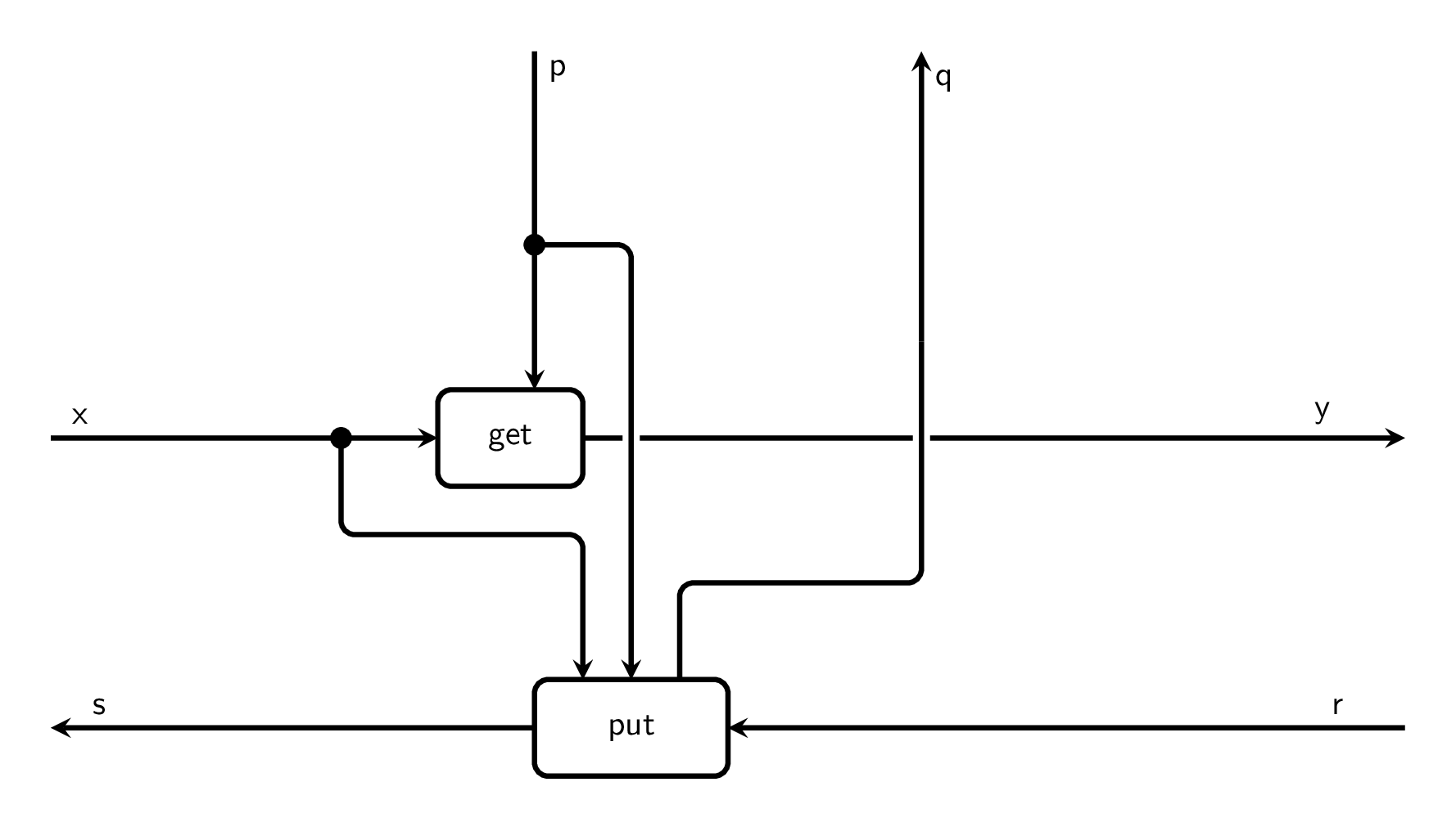
By looking at the internals of a lens and the direction of the arrows, it becomes clear that data flows in two different directions:

• The forward pass, i.e. the get function, is happening at the time a player can observe the state before interacting with the game.
• The backward pass, i.e. the put function, is happening “in the future”, after all players did their moves, and represents the stage in which payoffs are being computed and passed around.

To limit mental overload, the following definition of non-parametrized lens will also come useful later:

-- A (non-parametrized) `Lens` is a `ParaLens` with trivial parameters
type Lens = ParaLens () ()

-- Non-parametrized Lens constructor
nonPara :: (x -> y) -> (x -> r -> s) -> Lens x s y r
nonPara get put = MkLens (\_ x -> get x) (\_ x r -> (put x r, ()))

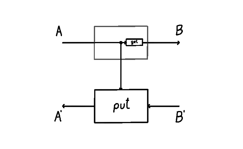
Diagrammatically we will represent wires of type () (the singleton type) as no wires at all. This will also come useful to us later in order to simplify some definitions and diagrams. For example, here’s a representation of the flow of data in a non-parametrized lens, courtesy of Bruno Gavranović:

Composing Lenses two ways

What makes Compositional Game Theory compositional is (unsurprisingly) the fact that parametrized lenses are closed under two different kinds of composition operators, one behaving like sequential composition of pure functions and one behaving like parallel execution of programs, or more or less like a tensor product³.

Sequential Composition

Let’s start with sequential composition: When the right boundary types of $\mathsf A:\binom{X}{S}\to\binom{Y}{R}$ match the left boundary types of $\mathsf B:\binom{Y}{R}\to\binom{Z}{T}$, we should be able to build another lens out of it that amounts to running what happens in $\mathsf A$ first, and then run what happens in $\mathsf B$ while taking into account the parameters of both lenses:

By trying to code this up in a type-directed way in Haskell, the only sensible definition that can possibly come out is the following:

infixr 4 >>>>

(>>>>) :: ParaLens p q x s y r -> ParaLens p' q' y r z t -> ParaLens (p, p') (q, q') x s z t
(MkLens get put) >>>> (MkLens get' put') =
  MkLens
    (\(p, p') x -> get' p' (get p x))
    (\(p, p') x t ->
      let (r, q') = put' p' (get p x) t
          (s, q) = put p x r
      in (s, (q, q'))
    )

From the Haskell implementation we can see that composing two lenses, parametrized or not, isn’t as simple as plugging one end into another, merging the parameter wires and calling it a day⁴. Something a bit more articulate is happening:

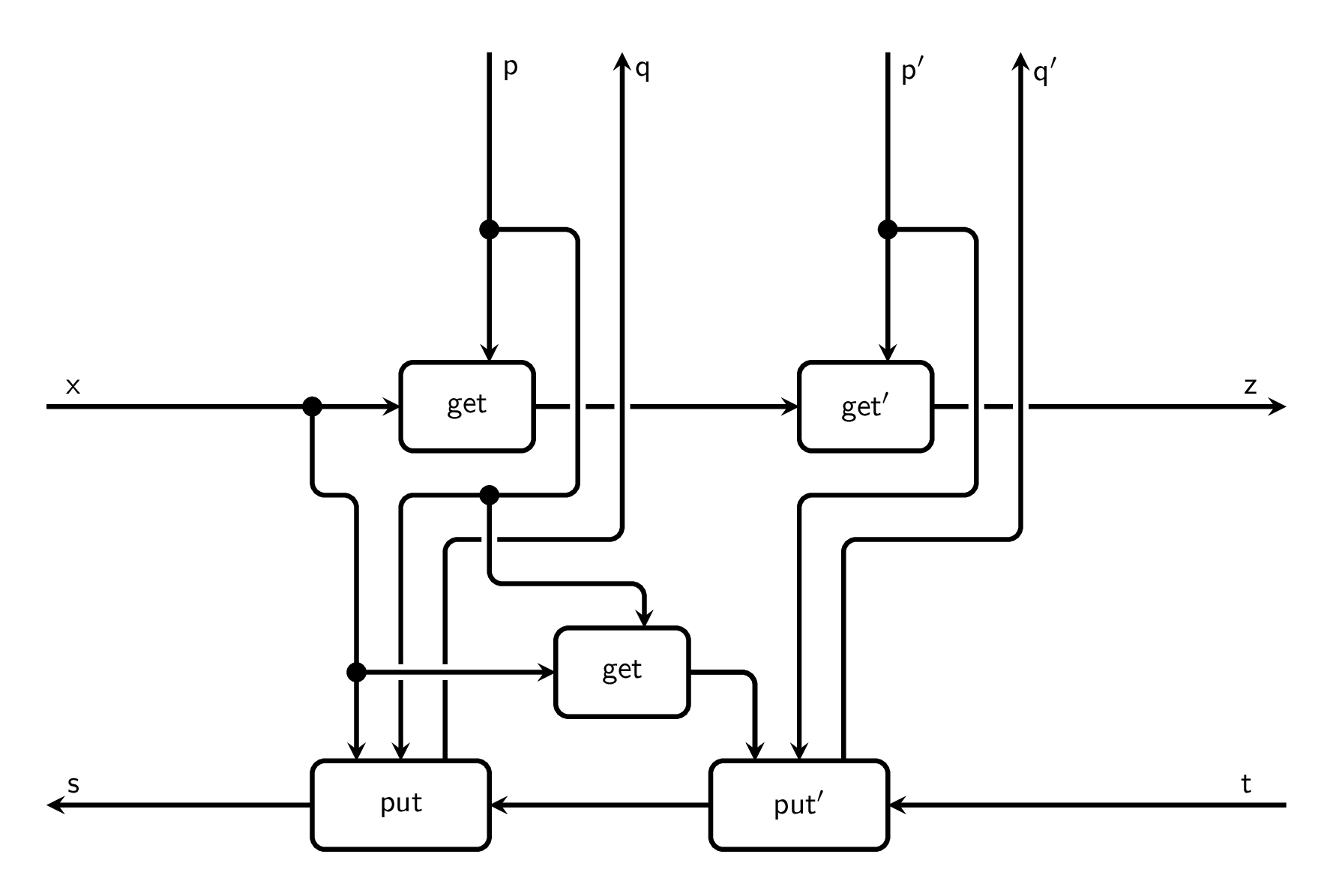
Mathematically, this amounts to the following compositions:

• For the get part: $P’\times P\times X\xrightarrow{\mathsf{id}\times\mathsf{get}}P’\times Y\xrightarrow{get’} Z$

• For the put part: \(\begin{align*} P'\times P\times X \times T &\xrightarrow{\mathsf{id}\times \Delta_{P}\times \Delta_{X}\times\mathsf{id}} P'\times P\times P\times X \times X \times T\\ &\xrightarrow{\mathsf{sym}\times \mathsf{get}\times \mathsf{sym}} P\times P'\times Y \times T \times X\\ &\xrightarrow{\mathsf{id}\times \mathsf{put}'\times \mathsf{id}} P\times R\times Q'\times X\\ &\xrightarrow{\mathsf{rearrange}} P\times X\times R\times Q'\\ &\xrightarrow{\mathsf{put}\times\mathsf{id}} S\times Q\times Q' \end{align*}\)

  Where $\Delta(x) = (x,x)$, $\mathsf{sym}(x,y)=(y,x)$ and $\mathsf{rearrange}$ is a suitable composition of $\mathsf{sym}$s.

Parallel Composition

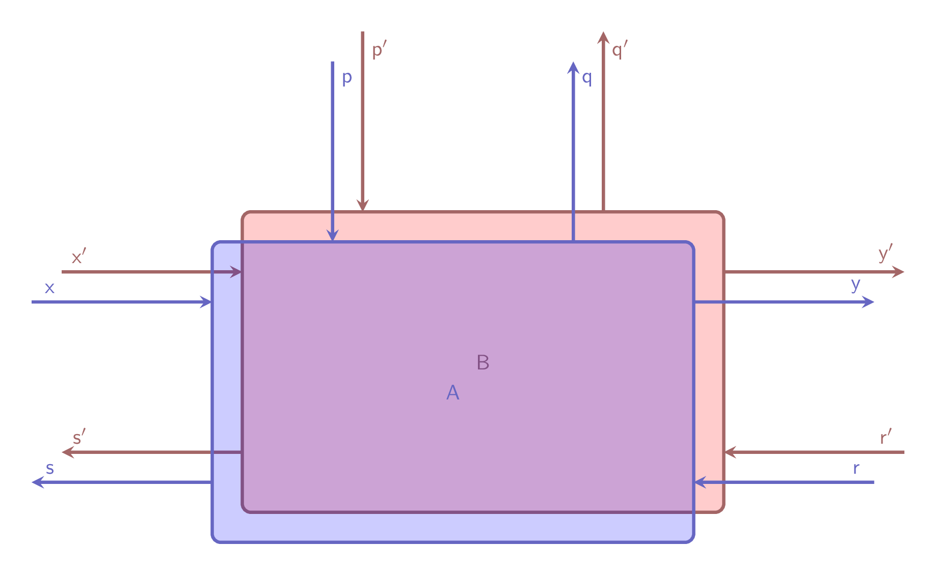
Luckily, parallel composition is way easier than the sequential one: In fact, parallel composition of $\mathsf{A}:\binom{X}{S}\to\binom{Y}{R}$ with parameters $\binom{P}{Q}$ and $\mathsf{B}:\binom{X’}{S’}\to\binom{Y’}{R’}$ with parameters $\binom{P’}{Q’}$, amounts to a lens $\mathsf{A}\times\mathsf{B}:\binom{X\times X’}{S\times S’}\to\binom{Y \times Y’}{R \times R’}$ with parameters $\binom{P\times P’}{Q \times Q’}$, such that \(\mathsf{put}_{\mathsf{A}\times\mathsf{B}}\) and \(\mathsf{get}_{\mathsf{A}\times\mathsf{B}}\) are respectively the cartesian product of the put and get functions from $\mathsf{A}$ and $\mathsf{B}$, modulo some rearrangement of inputs and outputs.

This is even clearer from the Haskell implementation:

infixr 4 ####

(####) :: ParaLens p q x s y r -> ParaLens p' q' x' s' y' r' -> ParaLens (p, p') (q, q') (x, x') (s, s') (y, y') (r, r')
(MkLens get put) #### (MkLens get' put') =
  MkLens
    (\(p, p') (x, x') -> (get p x, get' p' x'))
    (\(p, p') (x, x') (r, r') ->
      let (s, q) = put p x r
          (s', q') = put' p' x' r'
      in ((s, s'), (q, q'))
  )

Diagrammatically, this amounts to just putting the two lenses near each other.

Building Concrete Lenses

Now that we have laid all the groundwork, let’s have a look at a couple of concrete examples of lenses.

Lenses from Functions

Our first source of lenses will be functions: For each function $f: X\to S$ there is a non-parametrized lens $\mathsf{F}:\binom{X}{S}\to\binom{\mathbf{1}}{\mathbf{1}}$ such that $\mathsf{get}(*,x)=*$ and $\mathsf{put}(*,x,*)=(f(x),*)$. Vice-versa, we can always extract a unique function from non-parametrized lenses of this kind.

funToCostate :: (x -> s) -> Lens x s () ()
funToCostate f = nonPara (const ()) (\x _ -> f x)

costateToFun :: Lens x s () () -> (x -> s)
costateToFun (MkLens _ f) x = fst $ f () x ()

Similarly, for each function $f: P\to Q$ there is a parametrized lens \(\bar{\mathsf{F}}:\binom{\mathbf{1}}{\mathbf{1}}\to\binom{\mathbf{1}}{\mathbf{1}}\) with parameters \(\binom{P}{Q}\), such that $\mathsf{get}(*,*)=*$ and $\mathsf{put}(p,*,*)=(f(p),*)$. Likewise, we can always extract a unique function from this kind of parametrized lenses.

funToParaState :: (p -> q) -> ParaLens p q () () () ()
funToParaState f = MkLens (\_ _ -> ()) (\p _ _ -> ((), f p))

paraStateTofun :: ParaLens p q () () () () -> (p -> q)
paraStateTofun (MkLens _ coplay) p = snd $ coplay p () ()

Lenses from Scalars

For each value $\bar{y}\in Y$ and for any set $R$ we can build a non-parametrized lens \(\mathcal{S}_\bar{y}:\binom{\mathbf{1}}{\mathbf{1}}\to\binom{Y}{R}\) such that \(\mathsf{put}(*,*)=\bar{y}\) and \(\mathsf{get}(*,*,r)=(*,*)\).

scalarToState :: y -> Lens () () y r
scalarToState y = nonPara (const y) const

stateToScalar :: Lens () () y r -> y
stateToScalar (MkLens get _) = get () ()

The Identity Lens

The Identity Lens is a non-parametrized lens of type \(\binom{X}{S}\to\binom{X}{S}\) that serves as the identity morphism for parametrized lenses, i.e. pre-/post-composing a lens $\mathsf{A}$ with the identity lens gives you back $\mathsf{A}$ modulo readjusting the parameters (we will see how to do that in the next post). In Haskell:

idLens :: Lens x s x s
idLens = nonPara id (\_ x -> x)

Corners

(Right) Corners are parametrized lenses of type \(\binom{\mathbf{1}}{\mathbf{1}}\to\binom{Y}{R}\) and parameters $\binom{Y}{R}$ that bend parameter wires into right wires, such that \(\mathsf{get}(y,*)=y\) and \(\mathsf{put}(y,*,r)=(r,*)\).

corner :: ParaLens y r () () y r
corner = MkLens const (\_ _ r -> ((), r))

And diagrammatically:

As we will see in later posts, corners are an important component of bimatrix games.

Final Remarks

Parametrized lenses are not only useful for reasoning about Open Games, but also serve as the base of a whole categorical framework for reasoning about complex multi-agent systems which has also been applied to gradient-based learning, dynamic programming, reinforcement learning, bayesian inference and servers on top of various flavors of game theory (e.g.[2105.06763]). Indeed, this categorical framework is so general and promising that we spawned an entire research institute dedicated to it.

Phew! That’s all for today. I hope that this introduction to the world of parametrized lenses has left you wanting for more! I’ll see you in the next post, were we will explore how to handle spurious parameters with reparametrizations and model players and their agency with selection functions.